Seminar talk: Simulation-based Inference (SBI)#
- Date:
2026-03-16
- Tags:
bayes, simulation-based inference, SNPE, seminar
A seminar talk I gave alongside the special course in Simulation-based Inference that ran at Aalto in early 2026 — the same course that anchored the work in StimIQ, EASE Health, and QSVT4CRA.
SBI is the method I keep coming back to whenever a problem is hard to likelihood but easy to simulate. Instead of writing down \(p(x\mid\theta)\) analytically and inverting it, you:
Pick a forward model / simulator — encode the structure you understand.
Sample parameters \(\theta\sim p(\theta)\), run the simulator, observe \(x\sim p(x\mid\theta)\).
Train a neural posterior estimator (SNPE) — or an emulator, or a likelihood ratio network — directly on the \((\theta, x)\) pairs.
At inference time, condition on the observed data and let the amortised network give you \(p(\theta\mid x)\).
The slides work through:
Why SBI. Likelihood-free settings (stochastic simulators, agent-based models, implicit models) where MCMC is stuck because the likelihood isn’t a closed-form expression. The motivating examples are the ones I actually use: migraine risk under a mechanistic “digital shadow,” DBS parameter optimisation in Parkinson’s, credit-risk on the LUMI supercomputer.
The three families. Neural posterior estimation (SNPE-A/B/C), neural likelihood estimation (NLE), neural ratio estimation (NRE). When each one is the right tool.
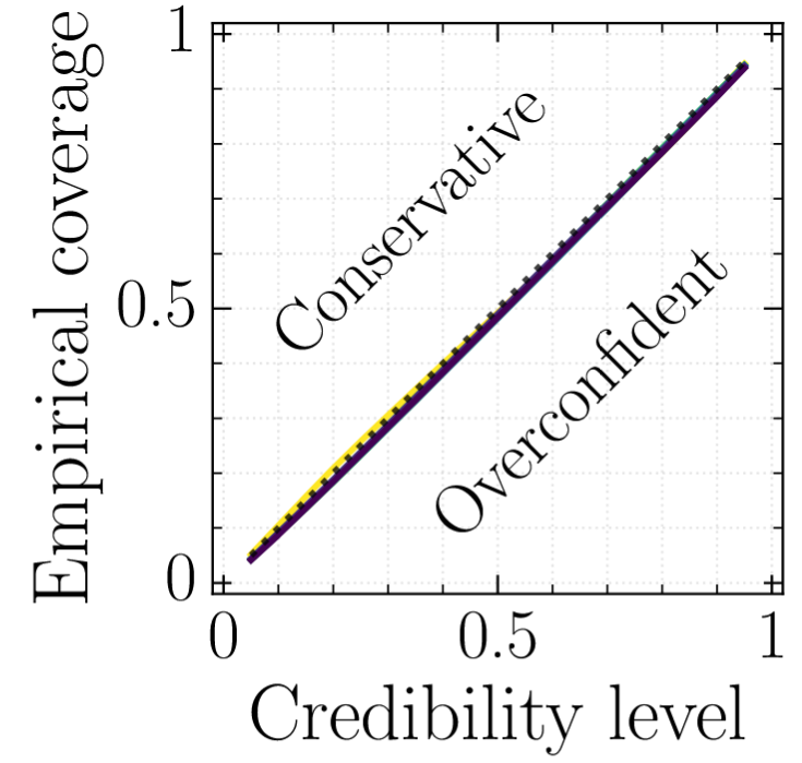
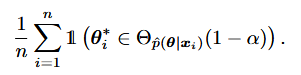
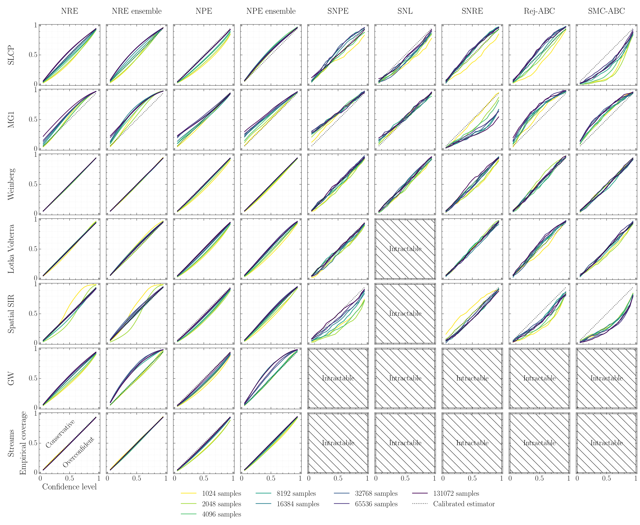
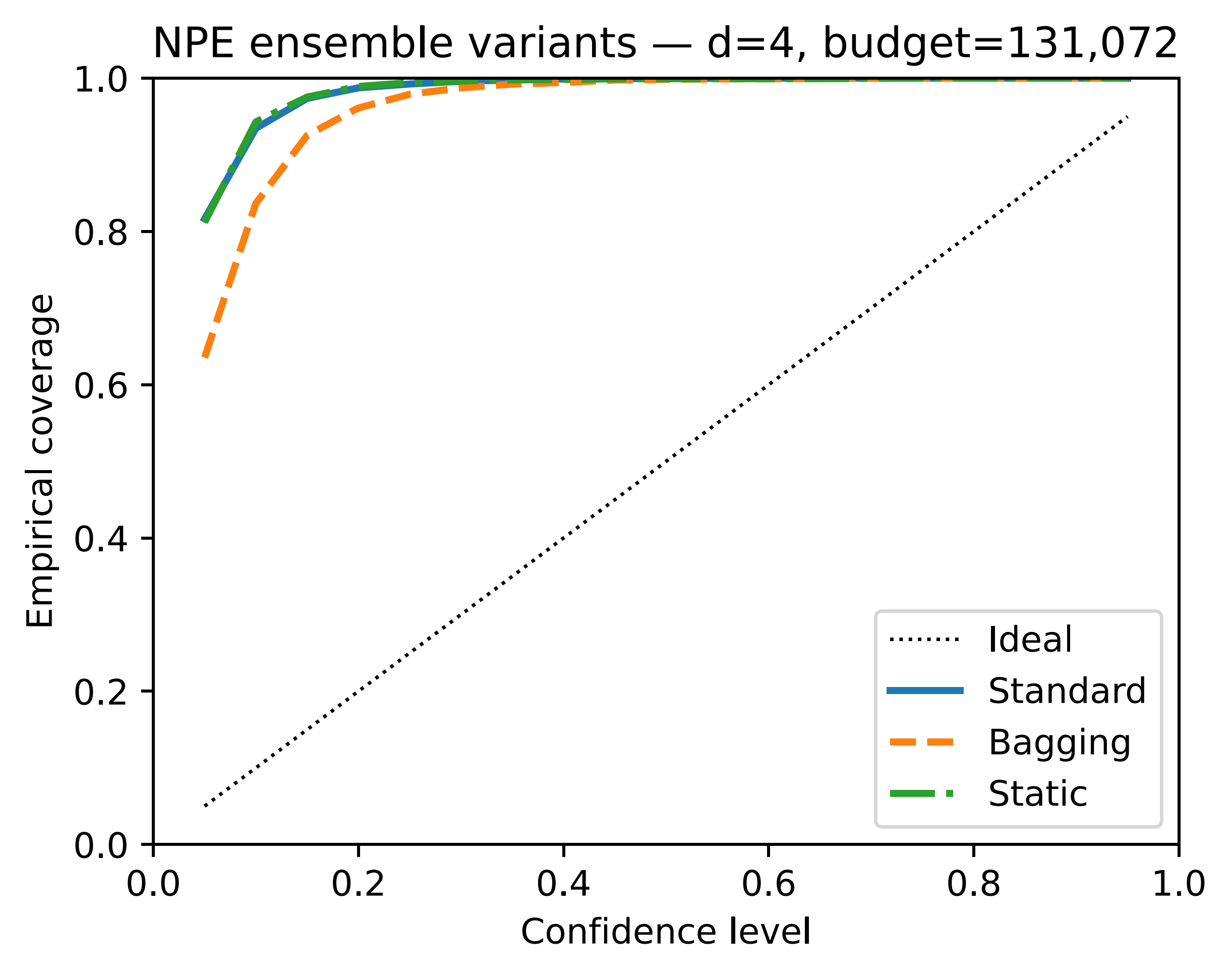
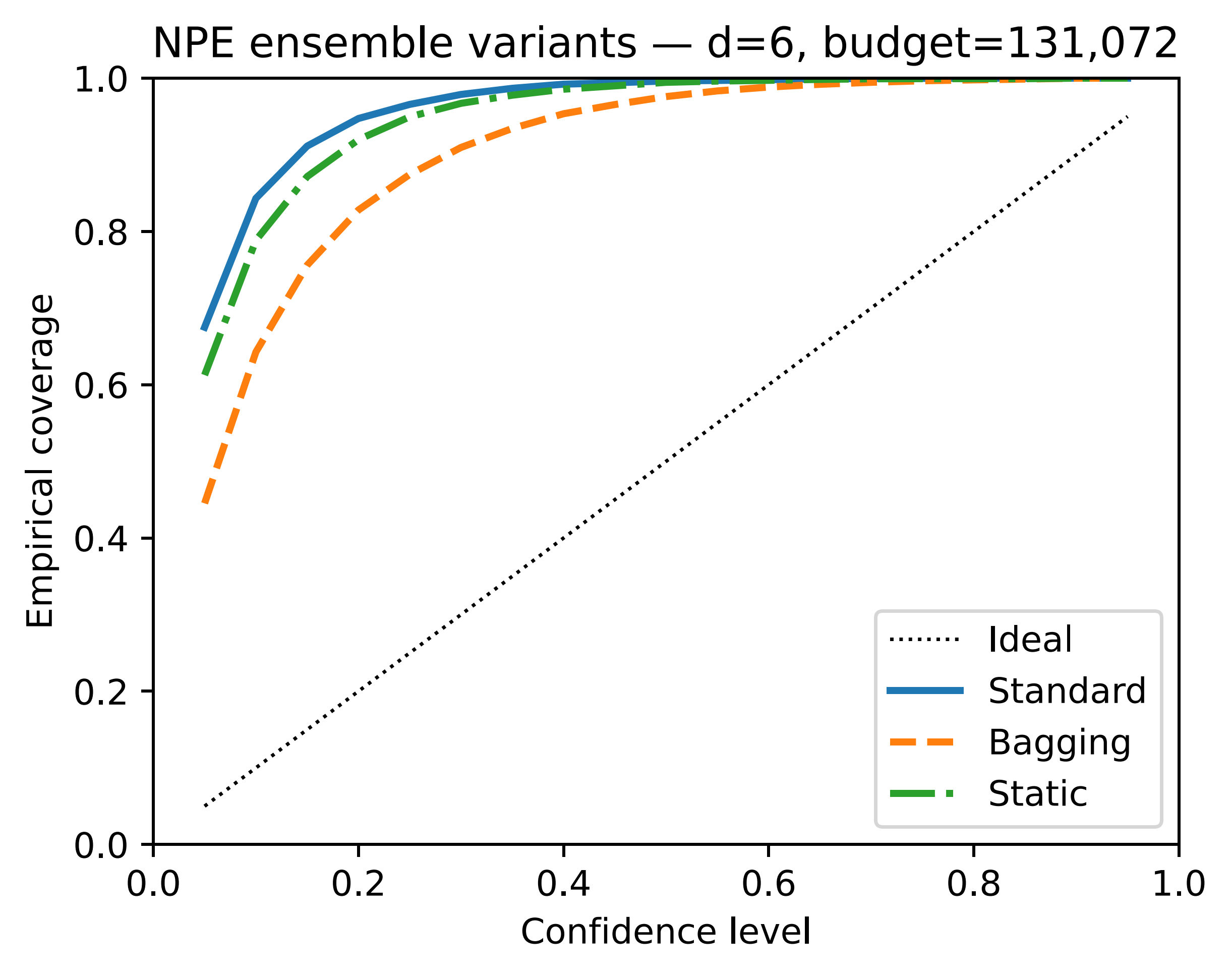
Calibration. A posterior isn’t useful if you can’t tell whether it’s honest. The calibration / coverage diagnostic on slide 8 — empirical coverage vs. credibility level — is the one I lean on. A well-calibrated posterior hugs the diagonal; an overconfident one falls below it.
The honest framing in the talk — and the one that shapes everything I build now — is that SBI is honest about what it doesn’t know. You get a full posterior, not a point estimate; and the simulator encodes your structural beliefs explicitly, so when the posterior is wide you can trace it back to a modelling choice.
Slides#
Slide 2 — the canonical SBI loop: simulate, train, condition.#

Slide 4.#
Slide 4.#

Slide 4.#
Slide 5.#
Slide 5.#
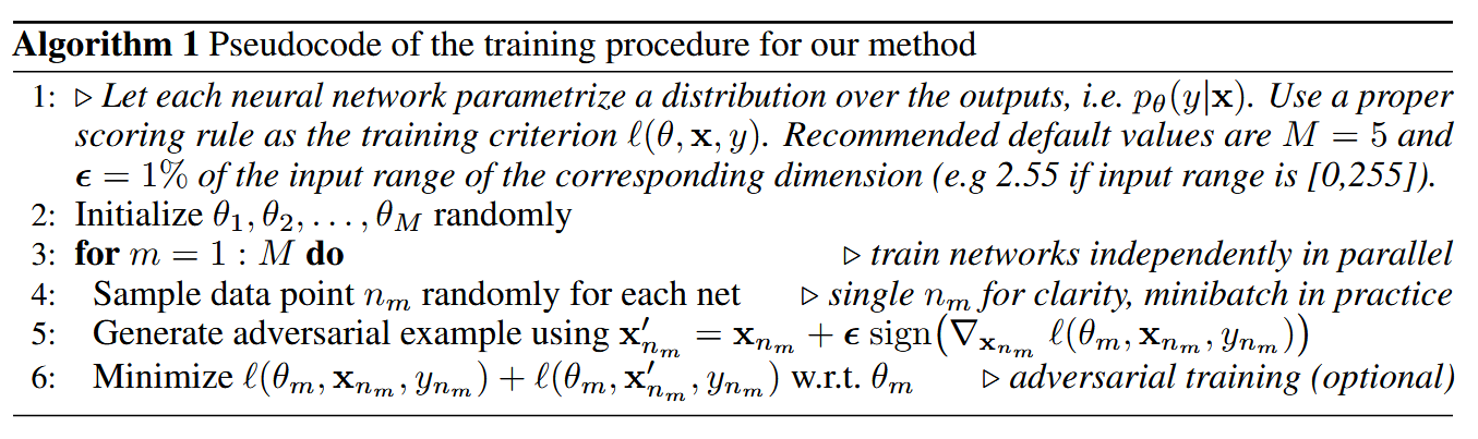
Slide 6.#
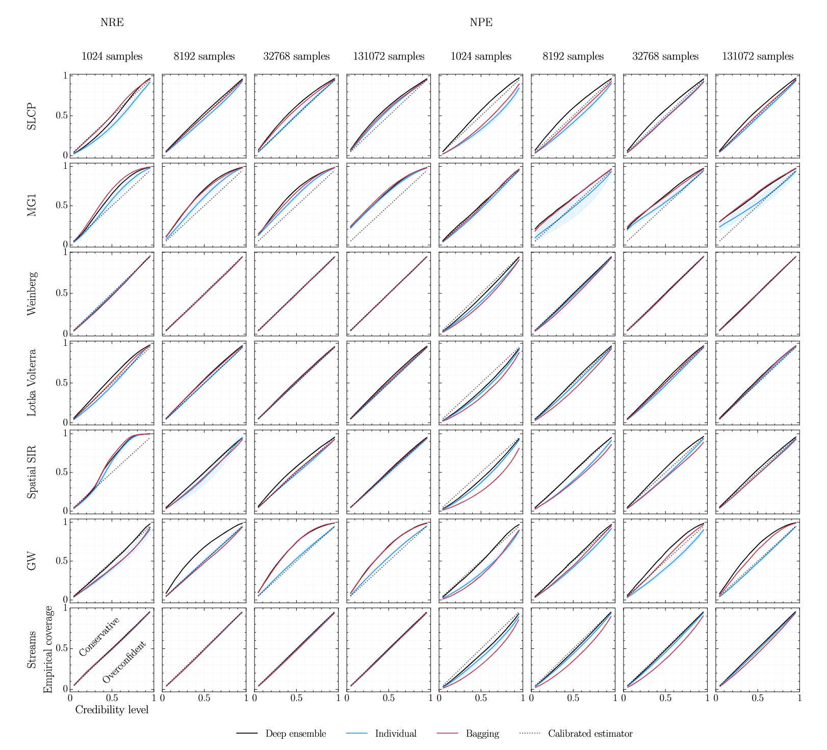
Slide 6.#
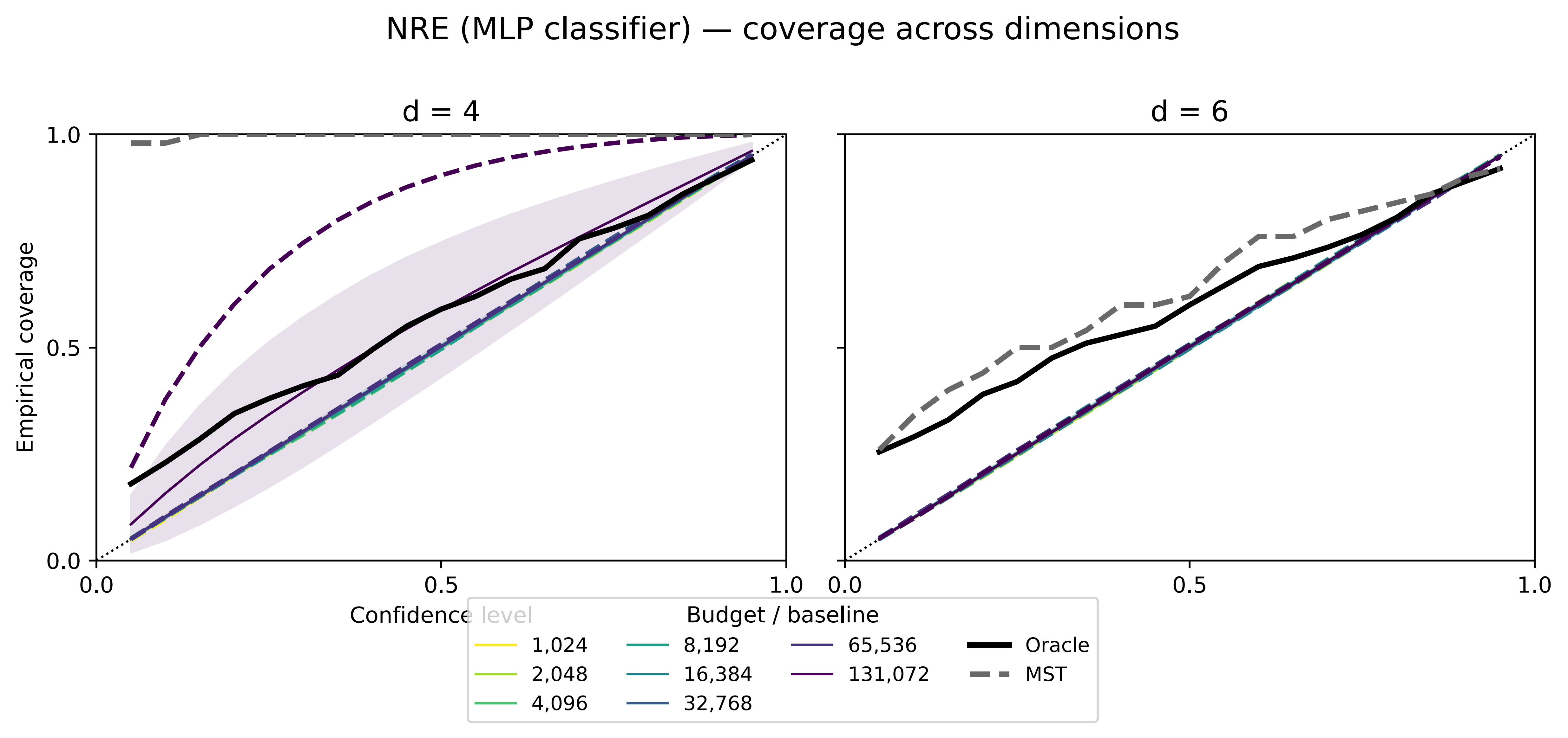
Slide 8 — empirical-coverage diagnostic. The yellow curve hugging the diagonal is a well-calibrated posterior; below it, the model is overconfident. This is the slide I keep coming back to.#
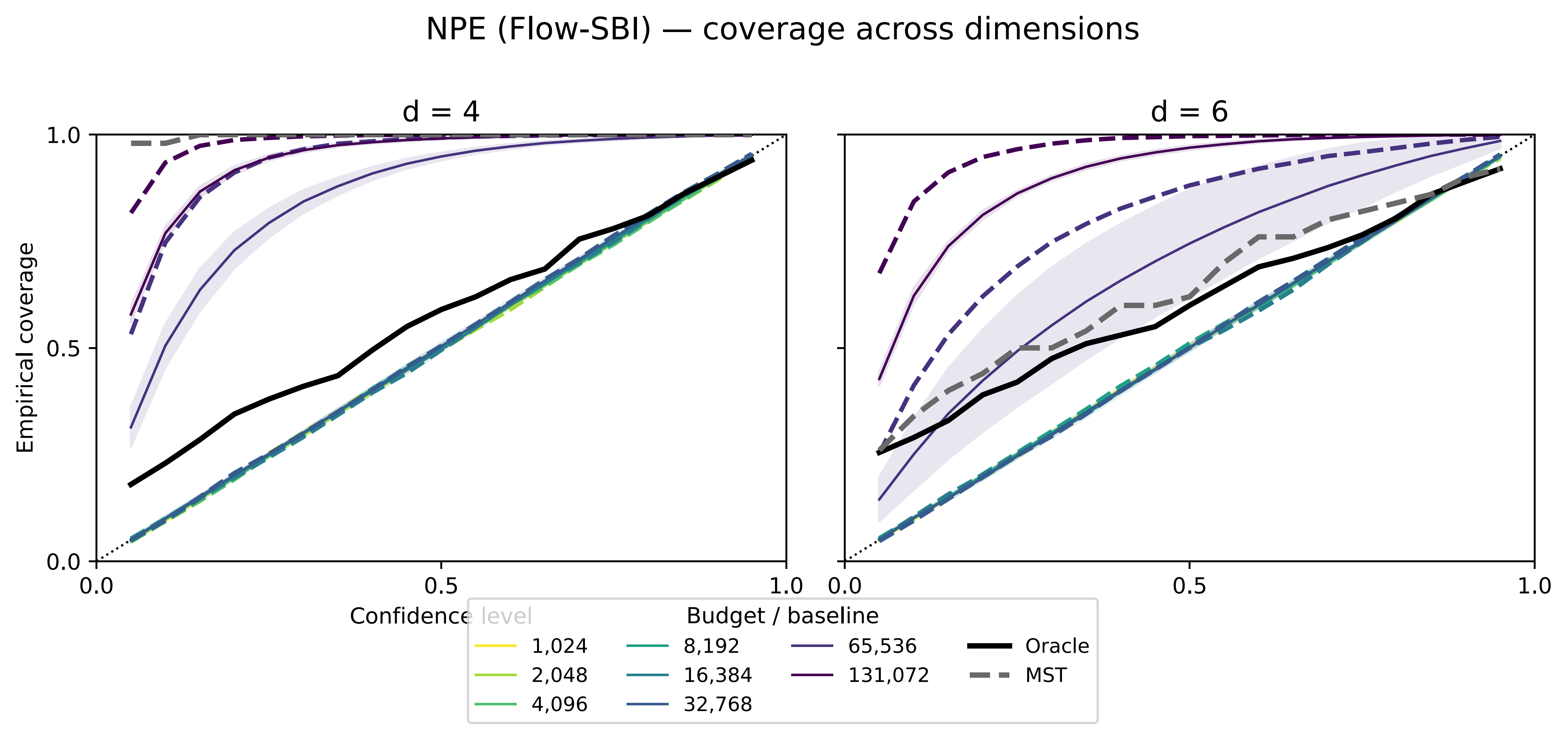
Slide 8.#
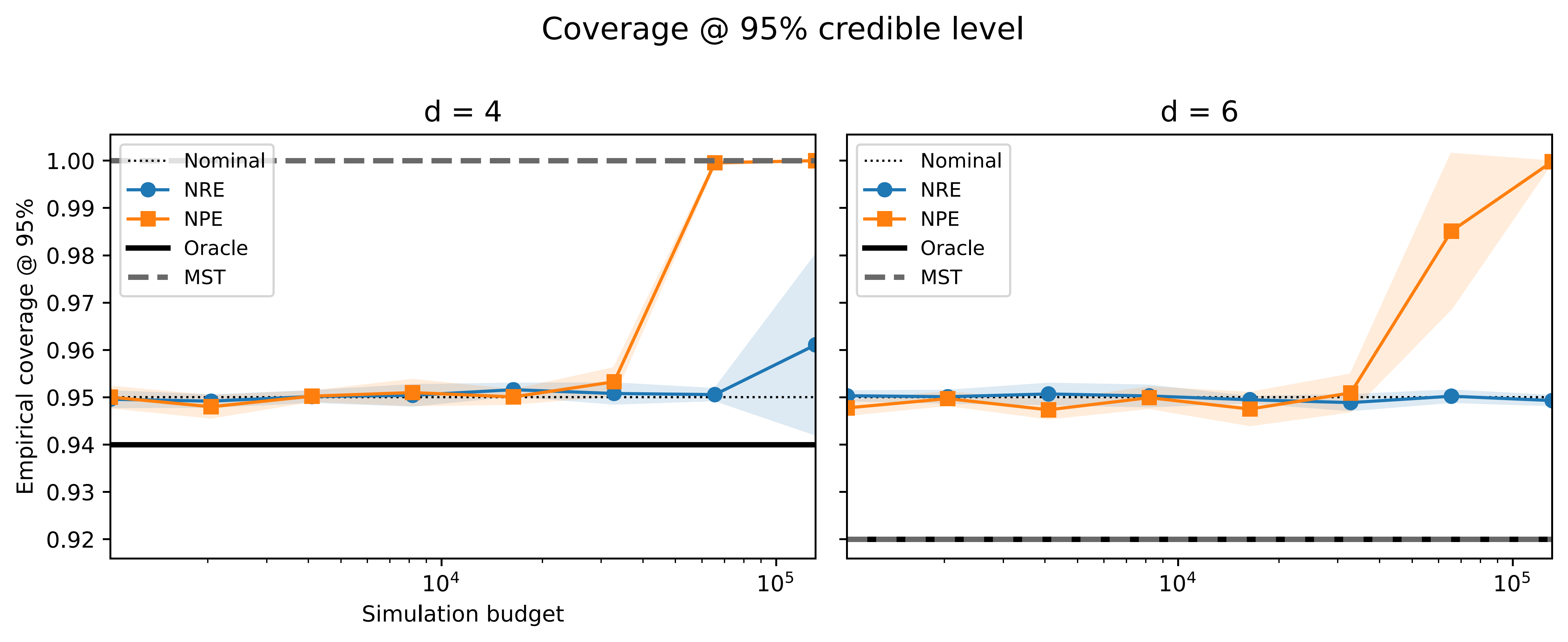
Slide 8.#
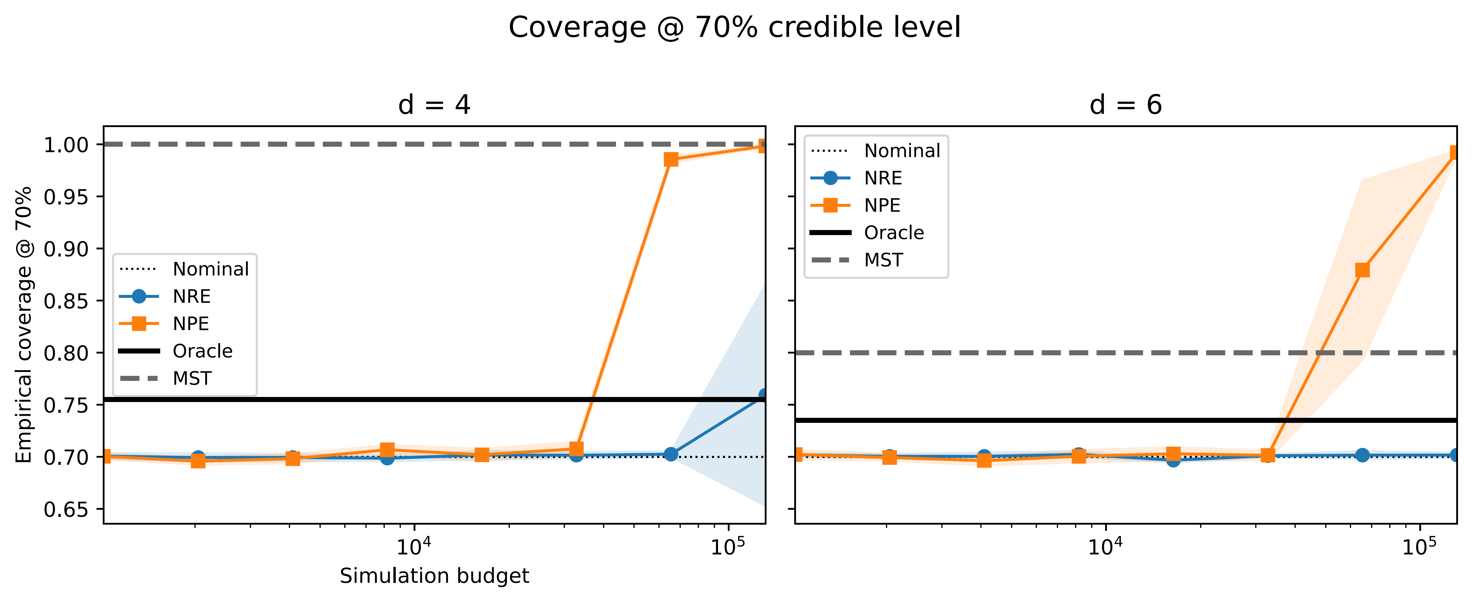
Slide 8.#
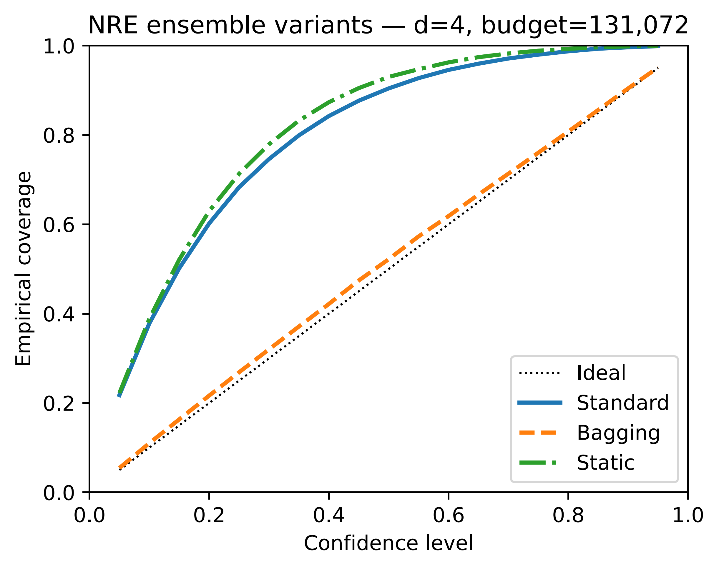
Slide 9.#
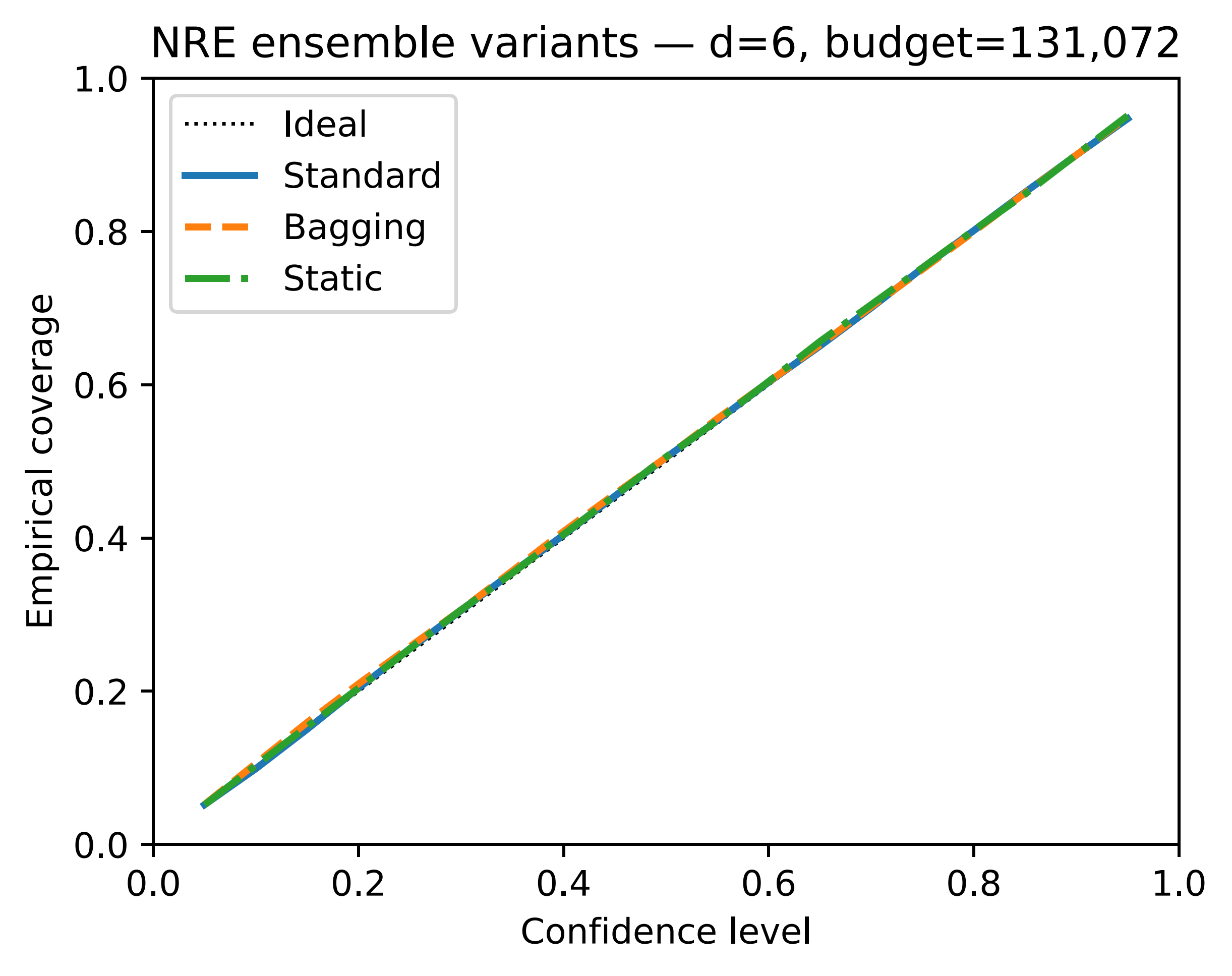
Slide 9.#
Slide 9.#
Slide 9.#
Slide 13.#
Slide 14.#
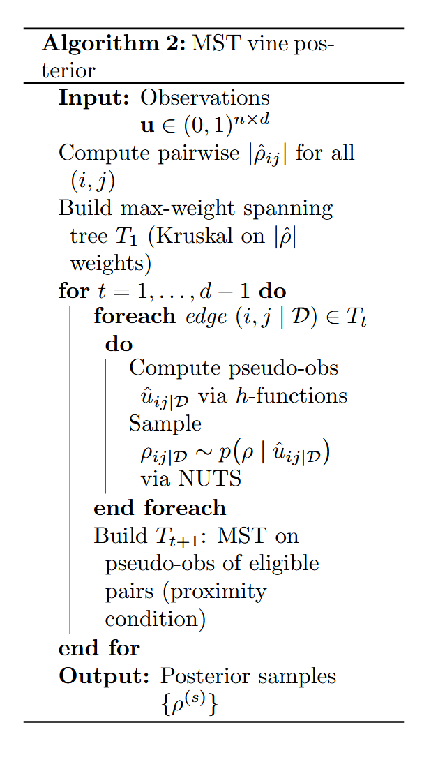
Slide 14.#
Links#
sbi library (the toolkit): https://www.mackelab.org/sbi/
Course context — the special course in Simulation-based Inference at Aalto (early 2026) that ran alongside the talk.