LIBS spectral processing
This chapter guides the reader on how to analyze data acquired with LIBS instruments. We will present the mathematics with simple graphs and algorithms implemented as MATLAB scripts. This is meant to be an easy to follow guide for the reader to try these methods themself and to understand how and why they work. By the end of this text you will have learned that LIBS data, even a big amount of data, can be managed and analyzed well with the right approaches. The examples used in this text are mostly measurements of rocks and minerals because that is what we work with daily, but the same methods can just as well be used for other materials.
Because of the nature of LIBS spectral data a multitude of different mathematical methods work well for processing and analysing LIBS measurements. The methods presented here are examples selected from those that in my own work experience have seemed to work well and which I am most familiar with. For more exhaustive listings of LIBS spectral analysis methods you can refer to multitude of sources for example [@ref-menetelmät1].
Spectral processing Part 1: LIBS analysis with pen and paper
We start with the simplest situation with a single spectrum obtained with a LIBS scanner when measuring a piece of rock that was labeled as. The spectrum is in figure 1, with frequency of measured light on X-axis and intensity count on Y-axis. In the spectrum we notice some couple of distinct high peaks, marked with arrows, some wider hill like shapes and some little up and downs all the time that look like random noise. The peaks are what is the most interesting for us so let's look at them. Dealing with the noise and continuum hills is the topic a few paragraphs later.
Imagine this graph printed on a millimeter paper and using ruler to measure the peak positions. Write the positions down to be later compared with reference book of atomic spectral lines. For fast identification you could also use printed see-through graphs of your reference materials or elements and overlay them on top of this graph to see which features match.
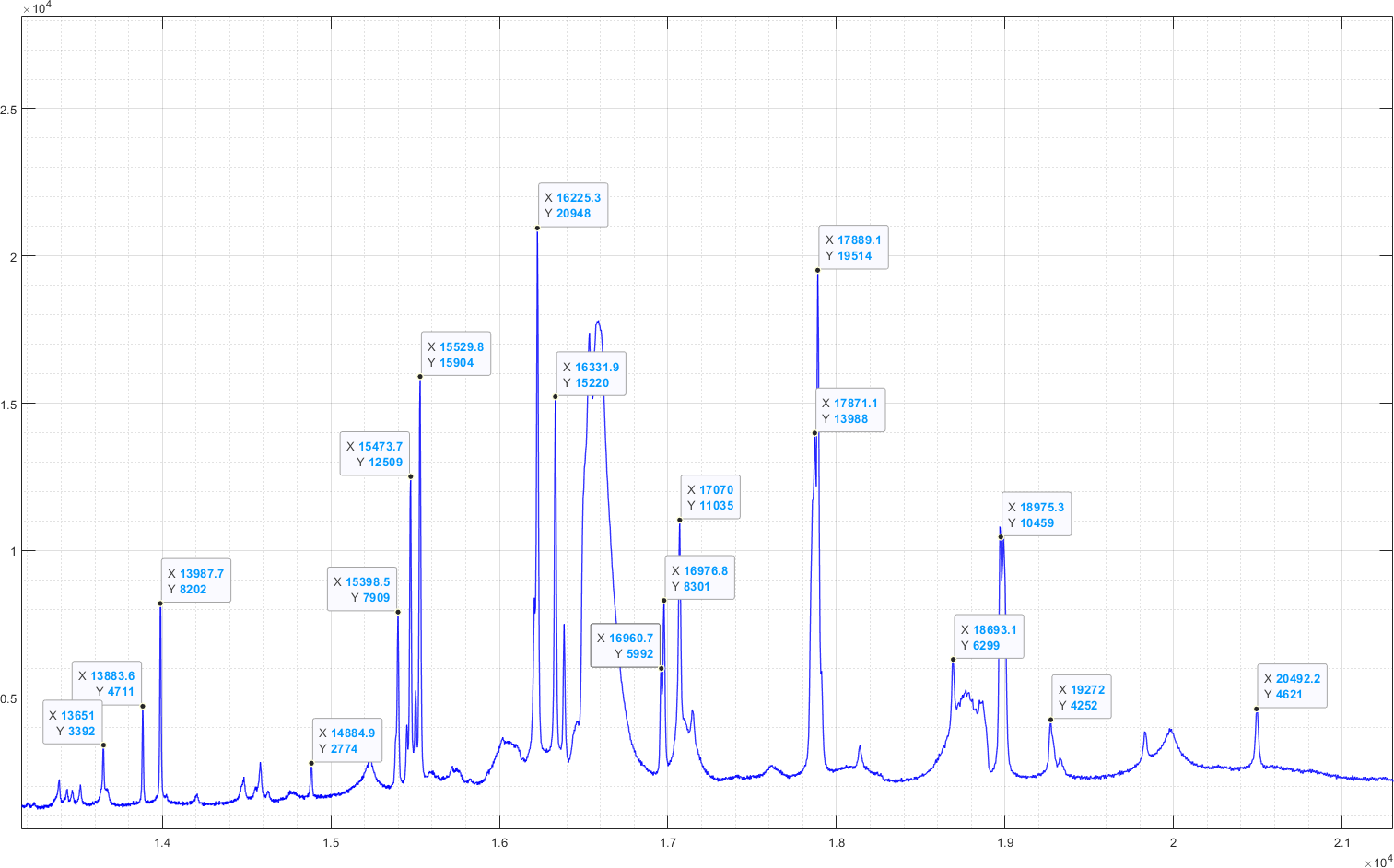
(figure note: We us here wavenumber(1/cm) instead of wavelength on the x-axis. Wavenumbers 13300-26300 correspond to visible light from red to violet (750-380nm), wavenumbers above 26300(<380nm) is ultraviolet and below 13300(>750nm) is infrared light. The wavenumber i.e. energy scale is chosen here for our mathematical operations to have clearer physical sense.)
Writing down the peak information
For a simple analysis these peaks are all we need to look at. We look at their wavenumber positions which corresponds to an excitation energy in the plasma, and their height which tells the intensity of each excitation. In this example we can gather the following list of peaks and their strengths:
peak 1, wavenum xx, intensity xx
peak 2, wavenum xx, intensity xx
peak 3, wavenum xx, intensity xx
peak 4, wavenum xx, intensity xx
peak 5, wavenum xx, intensity xx
How to interpret LIBS peaks?
We have a table of the excitation wavenumbers or energy levels in the plasma. Now comes the part of figuring out what these correspond to. At this point we need good references with a bit of good guessing of what elements we can realistically expect. Luckily we have great reference datasets build by others, such as VALD, Kurucz and NIST Atomic Spectral Database ASD Kramida, A, Yu Ralchenko, J Reader, and NIST ASD Team. ‘Atomic Spectra Database’. NIST, 2018.https://physics.nist.gov/asd. .
In this example we use a scraped LIBS peaks spreadsheet sourced from the NIST ASD. But the list contains tens of thousands of peaks so how do we know what to look for? Let's look at our example above and compare it to the peak list.
In mathematical terms
Let's calculate how much of the peak intensities our example spectrum come from each of the element. We do this by dividing the intensity values for each observed peak with the theoretical and then taking average for each element and dividing with the total for all elements. We get the following result:
peak_relative_strength = peak_observed / peak_expected_strength element_average = mean(peak_relative_strength for element) element_ratio = element_average
element 1, xx%
element 2, xx%
element 3, xx%
Because every elemental excitation, emission and absorption, behave differently and can depend on other elements present in the sample, these numbers do not directly correspond to concentration of the elements in the plasma but can give an approximation. At this point a qualitative result on how much of each element there is present is good enough for us. We will in later chapters look into how to calibrate this properly to get actual concentration numbers instead of peak intensity ratios.
Extending the same to the whole observed spectrum we have:
Spectral processing Part 2: LIBS analysis with computing
This chapter is about the computing tools we can use to process the spectra. For readers not interested in the technical details I suggest to jump over this chapter to move on to the conceptually more important methods in Spectral Processing Part 3.
What to do when I have not one but a million LIBS spectra?
Just do the same programmatically for all and then make you can make nice looking maps out of it. It will actually often times help the interpretation a lot, because more measurements, especially when tied with spatial information, can give us the required context to analyse the measurements better. The math involved is lightweight enough these analyses can easily be run on millions of points with modern computers. Examples of this are at LIBS visualization page.
Improving signal quality by removing noise and continuum and data compression
Noise removal and data compression
The signals we get are often noisy. The field of signal processing has many ways to improve the readability of noisy signals. We jump right on to a well working but not the easiest to understand method to approach this: wavelets. The reason for this is that wavelets are good not only for noise removal, but excellent for compressing LIBS data and sometimes useful for the analysis process as well!
To those who wish to understand wavelets or other signal processing methods to get the perfect signal digged out from a noisy mess of measurements, refer to the wikipedia article on them and to two excellent and freely available textbooks on signal processing: one by Orfanidis Orfanidis, Sophocles J. Optimum Signal Processing: An Introduction. 2nd ed., 2007. book available for free at http://eceweb1.rutgers.edu/~orfanidi/osp2e/ and second one by O’Haver O’Haver, T. A Pragmatic* Introduction to Signal Processing., 1995-2024, Book available for free at https://terpconnect.umd.edu/~toh/spectrum/index.html .
An example to illustrate much memory can be saved with compression, figure [f] shows a raw spectrum and then the same spectrum first compressed into wavelets and reproduced from that. In this example the wavelet representation uses xx% of the memory to store the spectrum.
The compression is not lossless so information is lost. But if the lost information is mostly noise we wanted to get rid of that anyway.
Continuum removal
To make interpretation of signal easier we can remove the continuum so the black body radiation and the broader expansions of the peaks themselves. Taking off the continuum reveals better those peaks that lie under the areas of other prominent features.
We use spline method to cut away the continuum. Figure [figuresplinematch] shows example of this process. Afterwards the resulting spectrum is "cleaner" looking and is easier to mathematically process. Be aware that this process does remove information from the spectrum such as the thermal radiation and more worryingly sometimes the shapes that might help us recognize molecular emission bands, example at molecular LIBS page. But for most purposes this cleaner up spectrum is a better fit and help us do comparisons between different spectra.
A simpler and easier to implement method that also works well to remove the continuum is calculating a moving minimum and removing that from the signal.
Peaks have width and we can model them as double-Lorentzians
Spectral processing part 3: Element concentrations and heatmaps
In this chapter we start making elemental maps. This and the next chapter present the imaging part of the LIBS imaging. These are the main techniques that I want to teach you about. Readers more interested in material or mineral classification without requiring to know the elements present can read Part 4 first and return to this chapter afterwards for details.
In first section we made a first analysis of a LIBS spectra. We found out the LIBS spectral peaks of our mystery sample and that this measurement is made from material containing elements x1 and x2. Now armed with more computing power and methods we can do our analysis better.
Find out the elements present
Quantifying the elemental content, qualitatively
We can extract intensity values from the set of elemental peaks and compare them to values for other elements.
Here it can help if the continuum has been removed from the signal before considering the peak heights. The peak height can be simply the intensity value at the pixel corresponding to the peak, or another option is to use more robust characteristics of the peak like peak width and shape. Here we use a calculated Lorentzian fit on the peak. Considering more than a single peak per element helps us bypass some issues with self absorption or saturated peaks but is of course mathematically more complex than comparing single values.
Note that if you want to implement these yourself you should start with simple methods. Just taking the pixel intensity values of the wavelengths for the peaks you want to consider is a fine working method in many applications.
Cut away elements from a spectrum
Gradient descent to find out proportions of all elements
Now we are ready for the automated computation process to find out all elements and their proportions.
Element concentrations: calibrate the element proportions
To get true elemental concentration values we need to use reference samples for which we know the concentrations i.e. they have been measured with a trustworthy method or they were specifically made as standard samples.
Here we have example of lithium standards of varying concentrations made for this purpose measured with LIBS
Elemental heatmaps
See more at chapter on LIBS visualization.
Spectral processing part 4: Minerals & Materials
This chapter we look at methods to directly quantify materials. Elemental analysis is the natural thing to do with LIBS data as most characteristic features visible in LIBS signal come from elemental emission peaks. But in many applications, knowing the elements is not the main thing we are after, often we just want to identify the material. This can be done by doing the elemental analysis from above and determining the material based on that, but often it is easier and better to not worry about the elements but directly look at mineral identification.
Interesting Features Finder IFF, to identify how many materials we have and what they look like
Interesting Features Finder IFF Wu, Q. et al. (2022) ‘Interesting features finder (IFF): Another way to explore spectroscopic imaging data sets giving minor compounds and traces a chance to express themselves’, Spectrochimica Acta Part B: Atomic Spectroscopy, 195, p. 106508. Available at: https://doi.org/10.1016/j.sab.2022.106508. is a computationally efficient method to approximate convex hull of large spectroscopic data. The great strength of IFF in comparison to most classifiers is that it gives a good chance for small trace features to pop out. It often highlights even a single pixel measurement of a remarkablably different signal so we don't miss any of the interesting features so to say.
What is convex hull and why do we want it?
Convex hull Convex hull wikipedia page https://en.wikipedia.org/wiki/Convex_hull. is the set of all of the datapoints that are on the outer corners of the data when represented in the 8000-dimensional space we have. So with spectroscopic data we have the conved hull has all the extreme cases and all of the other measurements can be represented as combinations of these. So in practice it gives us the most distinct spectral signal/ materials/minerals present in the data.
Calculating the true convex hull is not computationally feasible with any currently known methods for large multidimensional problems so we instead use an approximation created with the IFF method.
Let's run IFF
Spectral angle to classify measurement to materials
If we have a measurements of materials we know, let's say the fluorite and pyrite from above examples, we can use these as fingerprints to detect the same materials from any other measurement we have done.
Spectral angle mapping (SAM) Kruse, F.A. et al. (1993) ‘The Spectral Image Processing System (SIPS) Interactive Visualization and Analysis of Imaging Spectrometer Data’. is a good and computationally very fast method to compare the similarity of two measured spectra. Spectral angle between two measurements m1 and m2 is calculated simply by arccos(m1 dot m2), a small angle means that the measurements are highly similar. For a mathematical understanding of spectral angle calculations, consider each discrete wavelength as a dimension, then a measurement is a vector in this 8000-dimensional space and a spectral angle is the angle between two vectors, two measurements, in this space.
The quality of spectra angle mapping results depends strongly on couple of things that we should put effort on when we want the best results: first the quality of the reference datas and secondly the normalization methods on the raw spectral data. Thirdly subselecting only part of the data, such as considering only the parts of the spectrum where there are peaks important to our application, can significantly improve the results.
Make a map of minerals and quantify by point-counting
With IFF and SAM together, we can map the mineralogy. We use the resulting identified types from IFF and then use SAM to map each measurement point to the type closest or those with too much differing spectral angle we set as "unidentified".
Spectral processing part 5: Past the elemental peaks: Molecular LIBS, plasma properties and other signals in the spectrum
A LIBS spectrum contains more information than just the elemental excitations. Let's now look at all of those other features that we previously considered a nuisance and wanted to get rid of. What are they good for?
Spectral processing part 6: Textural and spatial processing
LIBS measurement setups are often not just for single measurements, but scanning setups that can acquire thousands or millions of measurement points from a single sample. Scanning LIBS or LIBS-imaging not only gives pretty pictures and all the information on nicely graphical form, it can also be used for new types of analyses.