Solving problems with CNF SAT solvers: The Sudoku example
We now show one example on how CF formulas and modern SAT solvers can be used to solve other computationally difficult problems. The following material is partly a recap from the Aalto courses CS-A1140 Data Structures and Algorithms and CS-E4800 Artificial Intelligence.
In a \(9 \times 9\) Sudoku, one has to complete a partially filled \(9 \times 9\) grid with the numbers \(1,...,9\) so that
each row contains the numbers \(1,...,9\),
each column contains the numbers \(1,...,9\), and
each of the disjoint \(3 \times 3\) sub-grids contain the numbers \(1,...,9\).
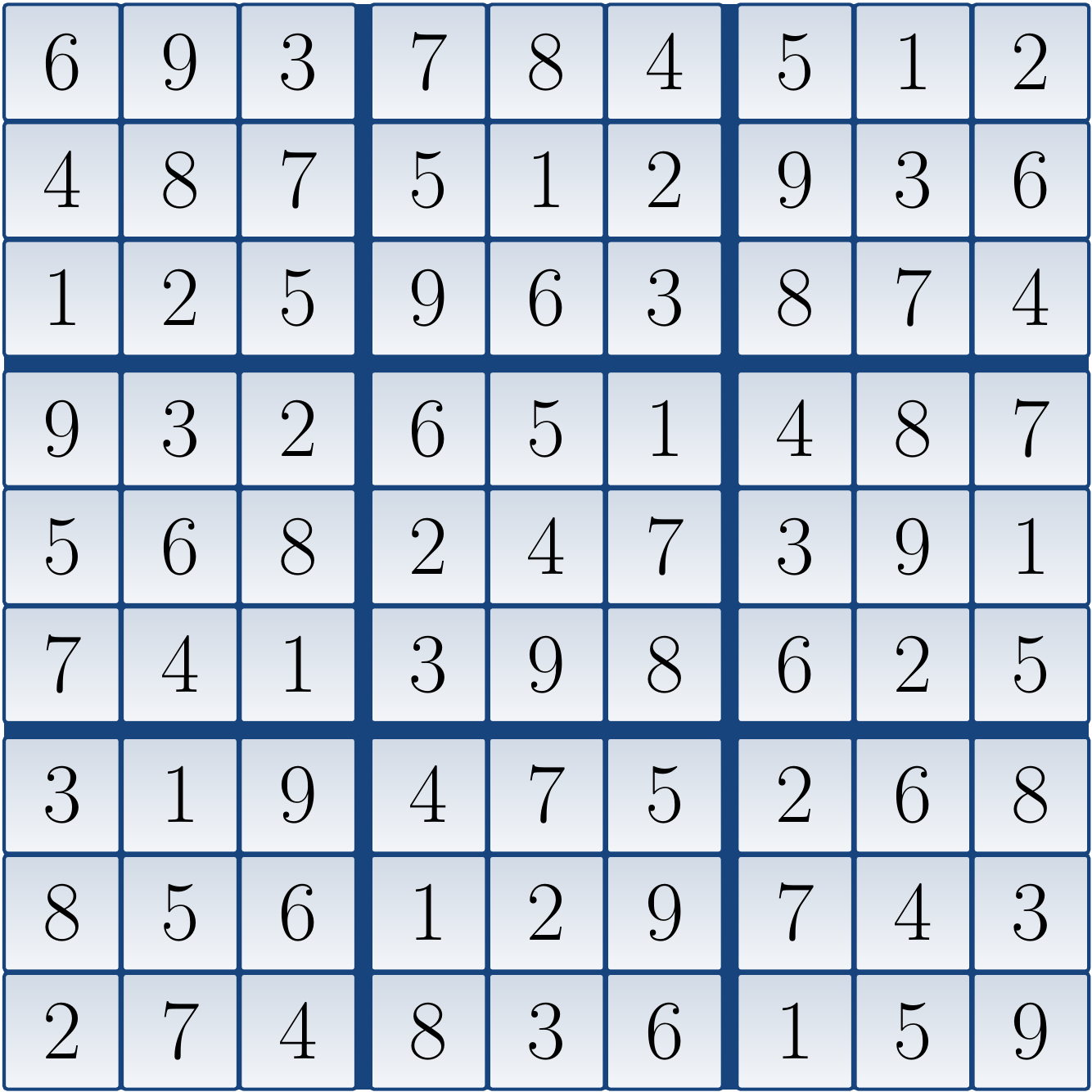
As an example, the unique solution to the Sudoku puzzle
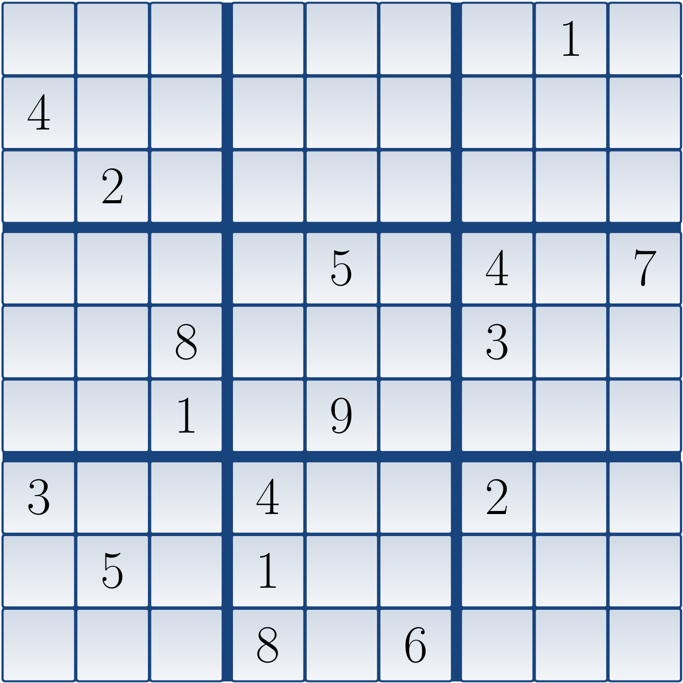
is
The Sudoku puzzle above is taken from Gordon Royle’s minimum Sudoku collection. It has 17 clues, puzzles with 16 or less clues do not exist (the solution for the puzzle must be unique).
In imperative and functional programming, Sudokus could be solved by programming a custom backtracking search algorithm (recall the “Recursion” round of CS-A1120 Programming 2). In constraint programming, however, we
encode the problem in a constraint language, and
let the constraint solver find the solution (or report that none exists).
In this first round, we use
propositional satisfiability as the constraint language, and
modern, highly efficient SAT solvers as the constraint solvers.
We thus reduce the problem of solving Sudokus to the propositional satisfiability problem and the work-flow looks like this:

Encoding Sudoku in CNF
Suppose that we are given an \(n \times n\) Sudoku puzzle, where the dimension \(n=d^2\) for some positive integer \(d\). Our goal is now to build a propositional formula \(\phi\) such that
the Sudoku puzzle has a solution if and only if the formula is satisfiable, and
from a satisfying assignment for \(\phi\) we can easily decode a solution for the Sudoku puzzle.
To obtain such a formula, we first introduce a variable
for each row \(r = [1..n]\), column \(c \in [1..n]\) and value \(v \in [1..n]\). The intuition is that if \(\SUD{r}{c}{v}\) is true, then the grid element at row \(r\) and column \(c\) has the value \(v\). To enforce that the values of the variables \(\SUD{r}{c}{v}\) model solutions to the Sudoku puzzle, the formula
is built by introducing sets of clauses that model different aspects of Sudoku solutions:
Each entry has at least one value: \(C_1 = \bigwedge_{r,c \in [1..n]}(\SUD{r}{c}{1} \lor \SUD{r}{c}{2} \lor ... \lor \SUD{r}{c}{n})\)
Each entry has at most one value: \(C_2 = \bigwedge_{r,c,v,v' \in [1..n] \textup{ with } v < v'}(\neg\SUD{r}{c}{v} \lor \neg\SUD{r}{c}{v'})\)
Each row has all the numbers: \(C_3 = \bigwedge_{r,v \in [1..n]}(\SUD{r}{1}{v} \lor \SUD{r}{2}{v} \lor ... \lor \SUD{r}{n}{v})\)
Each column has all the numbers: \(C_4 = \bigwedge_{c,v \in [1..n]}(\SUD{1}{c}{v} \lor \SUD{2}{c}{v} \lor ... \lor \SUD{n}{c}{v})\)
Each disjoint sub-grid has all the numbers: \(C_5 = \bigwedge_{r',c' \in [1..d], v \in [1..n]}(\bigvee_{(r,c) \in B_d(r'-1,c'-1)}\SUD{r}{c}{v})\) where \(B_d(r',c') = \Setdef{(r'd+i,c'd+j)}{i,j \in [1..d]}\)
The solution respects the given clues \(\SUDClues\): \(C_6 = \bigwedge_{(r,c,v) \in \SUDClues}(\SUD{r}{c}{v})\)
Note
Unlike in imperative programming, we do not give values for the variables, they are “unknowns”. It is the task of the constraint solver to find whether they can have some values that respect all the constraints (i.e., clauses in the case of CNF formula satisfiability).
The resulting formula has \(\Card{\SUDClues}\) unary clauses, \(n^2\frac{n(n-1)}{2}\) binary clauses, and \(4n^2\) clauses of length \(n\). Thus the size of the formula is polynomial in the grid dimension \(n\).
Example
Consider the Sudoku puzzle
The corresponding CNF formula is:
The DIMACS CNF file format
The DIMACS CNF format is a simple file format for storing CNF formulas. It is supported by practically all modern SAT solvers and it is also used in the regularly organized SAT Competitions that benchmarks the best solvers against each other. The format can be described as follows:
Lines starting with
care comments. The header line of form
p cnf n mdeclares that the problem consists of \(n\) variables \(x_1,...,x_n\) and \(m\) clauses. The following lines describe the clauses. A clause \((l_1 \lor l_2 \lor ... \lor l_k)\) is written as
v1 v2 ... vn 0, where each integer v\(i\) is (a) \(j\) if \(l_i\) is the positive literal \(x_j\), and (b) \(-j\) if \(l_i\) is the negative literal \(\neg x_j\), and
the last
0marks the end of the clause.
Example
The CNF formula
is given in the DIMACS representation as follows:
c Comments are ignored
p cnf 3 3
-1 2 0
-1 3 0
1 -2 -3 0
The DIMACS CNF format is not very nice for encoding problems by hand.
Thus one usually automatically generates such a file with some script program.
For instance, CNF instances for Sudoku puzzles could be generated by the following Python program sudoku-encode.py:
#!/usr/bin/python3
import sys
D = 3    # Subgrid dimension
N = D*D  # Grid dimension
if __name__ == '__main__':
    # Read the clues from the file given as the first argument
    file_name = sys.argv[1]
    clues = []
    digits = {'0':0,'1':1,'2':2,'3':3,'4':4,'5':5,'6':6,'7':7,'8':8,'9':9}
    with open(file_name, "r") as f:
        for line in f.readlines():
            assert len(line.strip()) == N, "'"+line+"'"
            for c in range(0, N):
                assert(line[c] in digits.keys() or line[c] == '.')
            clues.append(line.strip())
    assert(len(clues) == N)

    # A helper: get the Dimacs CNF variable number for the variable v_{r,c,v}
    # encoding the fact that the cell at (r,c) has the value v
    def var(r, c, v):
        assert(1 <= r and r <= N and 1 <= c and c <= N and 1 <= v and v <= N)
        return (r-1)*N*N+(c-1)*N+(v-1)+1

    # Build the clauses in a list
    cls = []  # The clauses: a list of integer lists
    for r in range(1,N+1): # r runs over 1,...,N
        for c in range(1, N+1):
            # The cell at (r,c) has at least one value
            cls.append([var(r,c,v) for v in range(1,N+1)])
            # The cell at (r,c) has at most one value
            for v in range(1, N+1):
                for w in range(v+1,N+1):
                    cls.append([-var(r,c,v), -var(r,c,w)])
    for v in range(1, N+1):
        # Each row has the value v
        for r in range(1, N+1): cls.append([var(r,c,v) for c in range(1,N+1)])
        # Each column has the value v
        for c in range(1, N+1): cls.append([var(r,c,v) for r in range(1,N+1)])
        # Each subgrid has the value v
        for sr in range(0,D):
            for sc in range(0,D):
                cls.append([var(sr*D+rd,sc*D+cd,v)
                            for rd in range(1,D+1) for cd in range(1,D+1)])
    # The clues must be respected
    for r in range(1, N+1):
        for c in range(1, N+1):
            if clues[r-1][c-1] in digits.keys():
                cls.append([var(r,c,digits[clues[r-1][c-1]])])

    # Output the DIMACS CNF representation
    # Print the header line
    print("p cnf %d %d" % (N*N*N, len(cls)))
    # Print the clauses
    for c in cls:
        print(" ".join([str(l) for l in c])+" 0")
The data files describing the actual puzzles are of the form illustrated
in the example file sudoku-royle.txt below.
.......1.
4........
.2.......
....5.4.7
..8...3..
..1.9....
3..4..2..
.5.1.....
...8.6...
Running the program on Linux with the clasp SAT solver, we get the following output.
python3 sudoku-encode.py sudoku-royle.txt | clasp -n 0
c clasp version 3.3.3
c Reading from stdin
c Solving...
c Answer: 1
v -1 -2 -3 -4 -5 6 -7 -8 -9 -10 -11 -12 -13 -14 -15 -16 -17 18 -19 -20 21
v -22 -23 -24 -25 -26 -27 -28 -29 -30 -31 -32 -33 34 -35 -36 -37 -38 -39
v -40 -41 -42 -43 44 -45 -46 -47 -48 49 -50 -51 -52 -53 -54 -55 -56 -57 -58
v 59 -60 -61 -62 -63 64 -65 -66 -67 -68 -69 -70 -71 -72 -73 74 -75 -76 -77
v -78 -79 -80 -81 -82 -83 -84 85 -86 -87 -88 -89 -90 -91 -92 -93 -94 -95
v -96 -97 98 -99 -100 -101 -102 -103 -104 -105 106 -107 -108 -109 -110 -111
v -112 113 -114 -115 -116 -117 118 -119 -120 -121 -122 -123 -124 -125 -126
v -127 128 -129 -130 -131 -132 -133 -134 -135 -136 -137 -138 -139 -140 -141
v -142 -143 144 -145 -146 147 -148 -149 -150 -151 -152 -153 -154 -155 -156
v -157 -158 159 -160 -161 -162 163 -164 -165 -166 -167 -168 -169 -170 -171
v -172 173 -174 -175 -176 -177 -178 -179 -180 -181 -182 -183 -184 185 -186
v -187 -188 -189 -190 -191 -192 -193 -194 -195 -196 -197 198 -199 -200 -201
v -202 -203 204 -205 -206 -207 -208 -209 210 -211 -212 -213 -214 -215 -216
v -217 -218 -219 -220 -221 -222 -223 224 -225 -226 -227 -228 -229 -230 -231
v 232 -233 -234 -235 -236 -237 238 -239 -240 -241 -242 -243 -244 -245 -246
v -247 -248 -249 -250 -251 252 -253 -254 255 -256 -257 -258 -259 -260 -261
v -262 263 -264 -265 -266 -267 -268 -269 -270 -271 -272 -273 -274 -275 276
v -277 -278 -279 -280 -281 -282 -283 284 -285 -286 -287 -288 289 -290 -291
v -292 -293 -294 -295 -296 -297 -298 -299 -300 301 -302 -303 -304 -305 -306
v -307 -308 -309 -310 -311 -312 -313 314 -315 -316 -317 -318 -319 -320 -321
v 322 -323 -324 -325 -326 -327 -328 329 -330 -331 -332 -333 -334 -335 -336
v -337 -338 339 -340 -341 -342 -343 -344 -345 -346 -347 -348 -349 350 -351
v -352 353 -354 -355 -356 -357 -358 -359 -360 -361 -362 -363 364 -365 -366
v -367 -368 -369 -370 -371 -372 -373 -374 -375 376 -377 -378 -379 -380 381
v -382 -383 -384 -385 -386 -387 -388 -389 -390 -391 -392 -393 -394 -395 396
v 397 -398 -399 -400 -401 -402 -403 -404 -405 -406 -407 -408 -409 -410 -411
v 412 -413 -414 -415 -416 -417 418 -419 -420 -421 -422 -423 424 -425 -426
v -427 -428 -429 -430 -431 -432 -433 -434 435 -436 -437 -438 -439 -440 -441
v -442 -443 -444 -445 -446 -447 -448 -449 450 -451 -452 -453 -454 -455 -456
v -457 458 -459 -460 -461 -462 -463 -464 465 -466 -467 -468 -469 470 -471
v -472 -473 -474 -475 -476 -477 -478 -479 -480 -481 482 -483 -484 -485 -486
v -487 -488 489 -490 -491 -492 -493 -494 -495 496 -497 -498 -499 -500 -501
v -502 -503 -504 -505 -506 -507 -508 -509 -510 -511 -512 513 -514 -515 -516
v 517 -518 -519 -520 -521 -522 -523 -524 -525 -526 -527 -528 529 -530 -531
v -532 -533 -534 -535 536 -537 -538 -539 -540 -541 542 -543 -544 -545 -546
v -547 -548 -549 -550 -551 -552 -553 -554 555 -556 -557 -558 -559 -560 -561
v -562 -563 -564 -565 566 -567 -568 -569 -570 -571 -572 -573 -574 575 -576
v -577 -578 -579 -580 581 -582 -583 -584 -585 -586 -587 -588 -589 -590 591
v -592 -593 -594 595 -596 -597 -598 -599 -600 -601 -602 -603 -604 605 -606
v -607 -608 -609 -610 -611 -612 -613 -614 -615 -616 -617 -618 -619 -620 621
v -622 -623 -624 -625 -626 -627 628 -629 -630 -631 -632 -633 634 -635 -636
v -637 -638 -639 -640 -641 642 -643 -644 -645 -646 -647 -648 -649 650 -651
v -652 -653 -654 -655 -656 -657 -658 -659 -660 -661 -662 -663 664 -665 -666
v -667 -668 -669 670 -671 -672 -673 -674 -675 -676 -677 -678 -679 -680 -681
v -682 683 -684 -685 -686 687 -688 -689 -690 -691 -692 -693 -694 -695 -696
v -697 -698 699 -700 -701 -702 703 -704 -705 -706 -707 -708 -709 -710 -711
v -712 -713 -714 -715 716 -717 -718 -719 -720 -721 -722 -723 -724 -725 -726
v -727 -728 729 0
s SATISFIABLE
c
c Models         : 1
c Calls          : 1
c Time           : 0.907s (Solving: 0.90s 1st Model: 0.81s Unsat: 0.09s)
c CPU Time       : 0.900s
Decoding it, we see that the first cell must have value 6, the second the value 9 and so on.
SAT Solver APIs
In addition to the DIMACS CNF file format, many SAT solvers also allow one to describe SAT problems via an API. For instance,
The MiniSat SAT solver has a rather clean C++ implementation and API and it is thus widely used in many applications and when developing new solver features
namespace Minisat {
class Solver {
public:
  Var newVar(bool polarity = true, bool dvar = true); // Add a new variable
  bool addClause(const vec<Lit>& ps); // Add a clause
  bool solve();  // Search without assumptions.
  ...
The Sat4j used in Round 10 of CS-A1140 Data Structures and Algorithms is implemented in Java and has a Java API.
The Z3 solver, that we use later in this course, allows also non-Boolean variables, linear equations etc and has bindings to .net, C, C++, Python, Java and OCaml.