A Theory Solver for Difference Logic¶

Recall that the difference logic is a syntactic restriction of linear arithmetic in which the atoms must be of the form \[x - y \bowtie c\] (or, equivalently, $ x \bowtie y + c $), where $ x $ and $ y $ are variables, $ c \in \Rats $, and $ \bowtie $ is $ = $, $ \neq $, $ < $, $ \le $, $ \ge $, or $ > $. That is, the atoms only restrict the difference between the variables $ x $ and $ y $. Both integer- and real-valued versions were defined:

$ \RDL $, Real Difference Logic, allows the variables to have real or rational values, while
$ \IDL $, Integer Difference Logic, restricts the values of the variables to be integers.

Example

The formula $$(x < y + 3) \land (y \le z+2) \land (z < x - 4)$$ is

$ \RDL $-satisfiable as, for instance, $ \Set{x \mapsto 1.5, y \mapsto -1, z \mapsto -3} $ is a model for it, but
$ \IDL $-unsatisfiable.

For simplicity, let us consider the integer version $ \IDL $; we discuss the $ \RDL $ case later in the subsection Handling the real/rational case. Furthermore, we normalize the atoms in the following way so that the difference logic solver only has to deal with atoms of the form $ x \le y + k $, where $ k $ is an integer constant, internally. First we do the following transformations:

The disequalities $ x \neq y + c $ are rewritten into $ ((x < y + c) \lor (x > y + c)) $ in the original formula level. After this, the SAT-solver part in the DPLL(T) solver takes care of “case splitting” and selects either (or both) of these atoms to be given to the difference logic solver.
Similarly, equalities of the form $ x = y + c $ are rewritten into $ (x \le y+c)\land(x \ge y + c) $.

After these, the CDCL SAT solver can assert atoms of the forms $ (x < y + c) $, $ (x \le y + c) $, $ (x \ge y + c) $, and $ (x > y + c) $ to the integer difference logic solver. As only atoms of the form $ (x \le y + k) $ for an integer $ k $ are handled in the underlying algorithm, the integer difference logic solver transforms the remaining cases to this form, when they asserted, as follows:

$ (x \le y + c) $ becomes $ (x \le y + \Floor{c}) $
$ (x \ge y + c) $ becomes $ (y \le x + \Floor{-c}) $
$ (x < y + c) $ becomes $ (x \le y + c - 1) $ if $ c $ is an integer and $ (x \le y + \Ceil{c}) $ otherwise
$ (x > y + c) $ becomes $ (y \le x - c - 1) $ if $ c $ is an integer and $ (y \le x + \Ceil{-c}) $ otherwise

From conjunctions to graphs¶

In our normalized setting described above, the task of an $ \IDL $-solver is thus to decide the satisfiability of conjunctions of the form \[\phi \Def (x_1 \le y_1 + k_1) \land … \land (x_n \le y_n + k_n)\] where $ x_i,y_i $ are some variables. One such solver can be obtained by associating $ \phi $ to the corresponding constraint graph $ \CG{\phi} $, which is a directed, edge-weighted graph such that

the vertex set consists of the variables in $ \phi $, and
for each atom $ (x_i \le y_i + k_i) $ in $ \phi $, $ \CG{\phi} $ has an edge from $ x_i $ to $ y_i $ with the weight $ k_i $. Such an edge will be denoted by $ {x_i} \DiffEdge{k_i} {y_i} $. in the following.

A path $ x’_1 \DiffEdge{k’_1} x’_2 … \DiffEdge{k’_m} x’_{m+1} $ for $ m \ge 2 $ in $ \CG{\phi} $ is a negative cycle if $ x’_{m+1} = x’_1 $ and $ \sum_{1 \le i \le m} k’_i < 0 $.

Theorem

A conjunction $ \phi $ of the normalized form above is satisfiable if and only if the constraint graph $ \CG{\phi} $ has no negative cycles.

Example: An unsatisfiable conjunction

Consider the conjunction \begin{eqnarray*} (x_1 \le x_3 - 6) \land (x_1 \le x_4 - 3) &\land&\\\\ (x_2 \le x_1 + 3) \land (x_3 \le x_2 + 2) &\land&\\\\ (x_3 \le x_4 - 1) \land (x_4 \le x_2 + 5). \end{eqnarray*} The constraint graph is

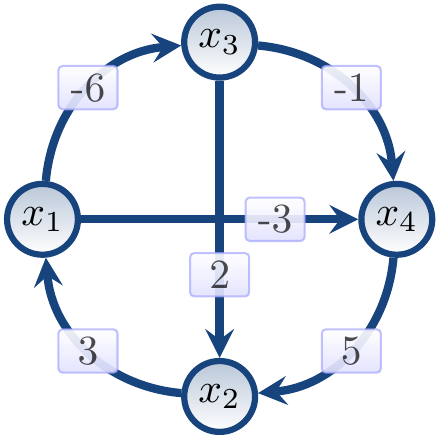
The graph has a negative cycle $ x_1 \to x_3 \to x_2 \to x_1 $. And in fact the conjunction is unsatisfiable by the following reasoning:

Take the atoms $ (x_1 \le x_3-6) $, $ (x_3 \le x_2+2) $ and $ (x_2 \le x_1+3) $ corresponding to the edges in the negative cycle.
$ (x_1 \le x_3-6) \land (x_3 \le x_2+2) $ implies $ x_1+6 \le x_3 \le x_2+2 $ and thus $ x_1 \le x_2-4 $.
$ (x_1 \le x_2-4) \land (x_2 \le x_1+3) $ implies $ x_1+4 \le x_2 \le x_1+3 $ and thus $ x_1 \le x_1-1 $ and $ 0 \le -1 $, which is a contradiction.

Example: A satisfiable conjunction

For the conjunction \begin{eqnarray*} &&(x_1 \le x_3 - 5) \land (x_1 \le x_4 - 3) \land\\\\ &&(x_2 \le x_1 + 3) \land (x_3 \le x_2 + 2) \land\\\\ &&(x_3 \le x_4 - 1) \land (x_4 \le x_2 + 5) \end{eqnarray*} the constraint graph is

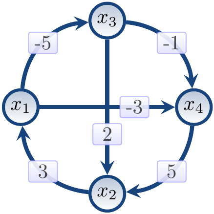
The constraint graph has no negative cycles and in fact \[\Set{x_1 \mapsto -2, x_2 \mapsto 1, x_3 \mapsto 3, x_4 \mapsto 4}\] is a model for the conjunction.

Therefore, in order to decide whether a normalized conjunction $ \phi $ is $ \IDL $-satisfiable, we can

build the constraint graph $ \CG{\phi} $, and
check whether $ \CG{\phi} $ has negative cycles.

Detecting negative cycles¶

How do we detect if a constraint graph has a negative cycle? One solutions is as follows:

Add an extra “root” vertex $ r $ to $ \CG{\phi} $ and an edge with weight $ 0 $ from it to each other vertex.
Run a single-source shortest path algorithm that is capable of detecting negative cycles for the root node $ r $.

One such negative-cycle deteting single-source shortest-path algorithm is the Bellman–Ford algorithm (recall the course CS-A1140 Data Structures and Algorithms). It works as follows. Each vertex $ x $ is associated with

an upper bound for the shortest distance $ \Dist{x} $ from the root $ r $ to $ x $, and
a link to the “parent” vertex in a shortest path.

Initially, $ \Dist{r} = 0 $ for the root vertex $ r $ and $ \Dist{x} = \infty $ for all the other non-root vertices. After this, iterate the following $ n $ times to compute the shortest distances:

For each edge $ x \DiffEdge{k} y $ in some order: if $ \Dist{x} + k < \Dist{y} $, then set $ \Dist{y} = \Dist{x} + k $ and set $ x $ to be the “parent” of $ y $.

At the end, a negative cycle exists if and only if $ \Dist{x}+k < \Dist{y} $ for some edge $ x \DiffEdge{k} y $. Of course, the above described algorithm is a basic version, optimizations do exists.

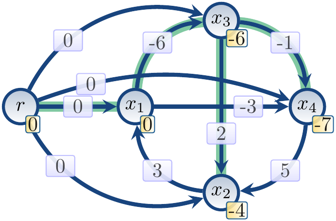
Example

Consider again the unsatisfiable conjunction \begin{eqnarray*} (x_1 \le x_3 - 6) \land (x_1 \le x_4 - 3) &\land&\\\\ (x_2 \le x_1 + 3) \land (x_3 \le x_2 + 2) &\land&\\\\ (x_3 \le x_4 - 1) \land (x_4 \le x_2 + 5). \end{eqnarray*} In the beginning, before the first iteration, the augmented constraint graph is the following, where the yellow boxes are the current upper bounds for the shortest distances from the root vertex $ r $.

After the first iteration, when the edges are relaxed in the lexicographical order, the distance upper bounds are as in the figure below. The parent vertex information is visualized by highlighting the edge whose source is the current parent of the target vertex.

After the second iteration, the situation is the following:

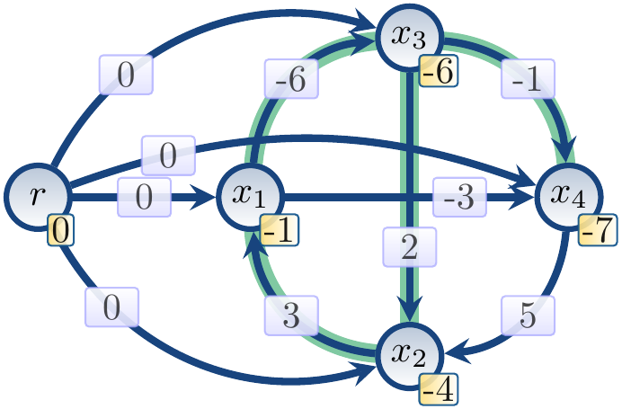
Finally, after the 5th iteration, the upper bounds are the following:

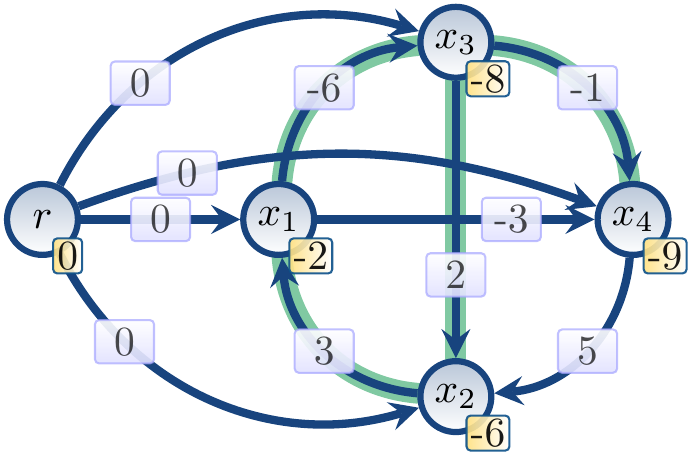
Now $ \Dist{x_2} + 3 < \Dist{x_1} $ and thus we have a negative cycle. We can find one such cycle by performing a depth-first search on the subgraph induced by the edges corresponding to the parent vertex pointers (the highlighted egdes in the figure).

Model construction¶

Assume that we have a satisfiable conjunction (again, in the normalized form). We can find a model for the conjunction as follows.

Run the Bellman–Ford algorithm on the augmented constraint graph. As the conjunction is satisfiable, the constraint graph does not have any negative cycles and therefore, for each vertex $ x $, $ \Dist{x} $ is the minimum distance from the root node $ r $ to $ x $ when the Bellman–Ford algorithm terminates.
After this, consider any equation $ x_i \le x_j + d_{i,j} $. It must hold that $ \Dist{x_i}+d_{i,j} \ge \Dist{x_j} $ because if $ \Dist{x_i}+d_{i,j} < \Dist{x_j} $, then $ \Dist{x_j} $ would not be the minimum distance from the root vertex. $ \Dist{x_i}+d_{i,j} \ge \Dist{x_j} $ is equal to $ \Dist{x_i} \ge \Dist{x_j}-d_{i,j} $, which in turn equals to $ -\Dist{x_i} \le -\Dist{x_j} + d_{i,j} $. Thus we get a model for the conjunction by taking \[x \mapsto -\Dist{x}\] for each variable $ x $.

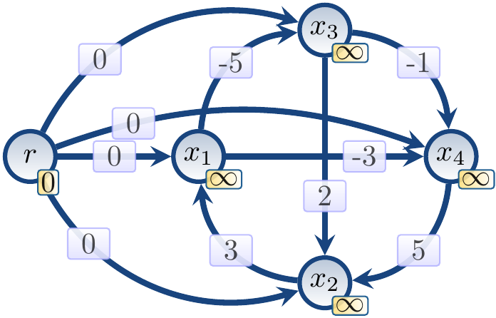
Example: A satisfiable conjunction

For the satisfiable conjunction \begin{eqnarray*} &&(x_1 \le x_3 - 5) \land (x_1 \le x_4 - 3) \land\\\\ &&(x_2 \le x_1 + 3) \land (x_3 \le x_2 + 2) \land\\\\ &&(x_3 \le x_4 - 1) \land (x_4 \le x_2 + 5) \end{eqnarray*} the augmented constraint graph in the beginning is

After the first iteration, the distance upper bounds are the following:

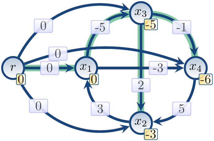
Now $ w(x_i) + d_{i,j} \ge w(x_j) $ for each edge $ x_i \DiffEdge{d_{i,j}} x_j $ and the upper bounds are the exact distances. From the distances, we get the model $ \Set{x_1 \mapsto 0, x_2 \mapsto 3, x_3 \mapsto 5, x_4 \mapsto 6} $ by using the construction described above.

Theory Implied Literals¶

Recall that theory implied literals are the literals whose truth value the theory solver can deduce based on the values of the literals asserted to it earlier. In the case of difference logic, observe that

$ x \le y + c $ implies $ x \le y + c’ $ for all $ c’ \ge c $, and
$ (x_1 \le x_2 + c_1) \land (x_2 \le x_3 + c_2) \land … \land (x_{n-1} \le x_n + c_{n-1}) $ implies $ x_1 \le x_n + \sum_{1 \le i \le {n-1}}c_i $.

Example

Consider again the satisfiable conjunction of difference logic atoms \begin{eqnarray*} \phi &=&(x_1 \le x_3 - 5) \land (x_1 \le x_4 - 3) \land\\\\ &&(x_2 \le x_1 + 3) \land (x_3 \le x_2 + 2) \land\\\\ &&(x_3 \le x_4 - 1) \land (x_4 \le x_2 + 5) \end{eqnarray*} Now $ \phi $ implies $ x_1 \le x_2 - 1 $ because $ (x_1 \le x_3 - 5) \land (x_3 \le x_2 + 2) $ implies $ (x_1 + 5 \le x_3 \le x_2 + 2) $ and thus $ (x_1 \le x_2 - 5 + 2) $ and $ (x_1 \le x_2 - 1) $.

From the above observation, we directly get the following:

Theorem

Given a satisfiable conjunction $ \phi $ and an atom $ x \le y + c $, $$\phi \IDLEntails (x \le y + c)$$ if and only if $ \CG{\phi} $ has a path from $ x $ to $ y $ with weight $ c $ or less.

This means that we can find all the implied atoms by computing all the shortest paths between the vertices in $ \CG{\phi} $. This can be done with, e.g., the Floyd–Warshall algorithm. The explanation of an implied atom $ x \le y + c $ is the conjunction of the atoms corresponding to the shortest path from $ x $ to $ y $.

Handling the real/rational case¶

So far we assumed integer-valued solutions, i.e., the logic $ \IDL $. What about $ \RDL $ allowing real-valued solutions? For that logic, one can use the approach in A. Armando, C. Castellini, E. Giunchiglia, M. Maratea: A SAT-Based Decision Procedure for the Boolean Combination of Difference Constraints, Proc. SAT 2004, pp 16–29. The idea is that the “problematic” conjunctions of the form $ x < y + c $ are rewritten into $ x \le y + c’ $, where $ c’ = c - \frac{1}{10^p(n^2+1)} $, $ n $ is the number of variables in the difference logic atoms, and $ p $ is the maximal number of digits appearing the right-hand side of the decimal points in the constants of the difference logic atoms. After this, a graph-based algorithm similar to the one described above can be used.

Some further reading¶

A. Armando, C. Castellini, E. Giunchiglia, M. Maratea: A SAT-Based Decision Procedure for the Boolean Combination of Difference Constraints, Proc. SAT 2004, pp 16–29
R. Nieuwenhuis and A. Oliveras: DPLL(T) with Exhaustive Theory Propagation and Its Application to Difference Logic, Proc. CAV 2005, pp. 321–334
S. Cotton and O. Maler: Fast and Flexible Difference Constraint Propagation for DPLL(T), Proc. SAT 2006, pp 170–183
S. Lahiri, M. Musuvathi: An Efficient Decision Procedure for UTVPI Constraints, Proc. FroCoS 2005, pp 168–183

Negative-cycle detection algorithms:

B. Cherkassky, A. Goldberg: Negative-cycle detection algorithms, Math. Program. 85(2):277–311, 1999