Constraint Propagation
We have already seen constraint propagation in action, but let’s define it bit more precisely.
The basic step in constraint propagation is called filtering a constraint. As input, filtering takes a constraint and the current domains for its variables. It then tries to remove all the values in the domains that do not appear in any solution to that constraint. That is, it tries to reduce the domains so that all the solutions are preserved. Thus “constraint filtering” in CSPs corresponds to a “unit clause propagation” step in CNF SAT solvers, but it is usually more complex because the domains are larger and the constraints are more complex. Filtering on the global constraint level can also be more effective than unit clause propagation in pruning the search space.
Constraint propagation then means the process of applying filtering to the constraints in the CSP instance at hand. As filtering one constraint can reduce the domains of its variables, it can trigger further reduction when filtering another constraint that also involves the reduced-domain variables. Thus a constraint can be filtered multiple times during the constraint propagation process. Usually the process is run to the end, meaning until no more reduction happens in filtering any of the constraints. Or if this takes too long, then until some resource usage limit is exceeded.
Let’s define constraint filtering more mathematically. As input, it takes
a constraint \( \Constr \subseteq \Dom{\CVarI1} \times \ldots \times \Dom{\CVarI k} \), and
the current domains \( \DomA{\CVarI i} \subseteq \Dom{\CVarI i} \) for \( i \in [1..k] \).
It then produces new domains \( \DomB{\CVarI i} \subseteq \DomA{\CVarI i} \) for all \( i \in [1..k] \) such that $$\Constr \cap (\DomA{\CVarI1}\times \ldots \times \DomA{\CVarI k}) = \Constr \cap (\DomB{\CVarI1}\times \ldots \times \DomB{\CVarI k}).$$
Example
When \( \DomA{x} = \Set{1,2,4} \) and \( \DomA{y} = \Set{1,2,5} \), filtering the constraint \( x = y \) optimally gives to domains \( \DomB x = \Set{1,2} \) and \( \DomB y = \Set{1,2} \). This is because the solutions of the constraint are \( x=1,y=1 \) and \( x=2,y=2 \).
Whenever feasible, our goal is to reduce the domains so that the constraint in question becomes arc-consistent.
Definition: Arc consistency of a constraint
A constraint \( \Constr \) is generalized arc consistent in the domains \( \Dom{\CVarI1},…,\Dom{\CVarI k} \) if, for every \( i \in [1..k] \) and every \( \Val \in \Dom{\CVarI i} \), there exists a tuple \( \Tuple{\ValI 1,…,\ValI k} \in \Constr \) such that \( \ValI i = \Val \).
We usually omit “generalized” and just use the term arc consistent (the term “arc consistency” is sometimes used for “generalized arc consistency” when the constraint is binary (i.e., over two variables)).
Example
Assume two variables, \( x \) and \( y \), and the domains \( \Dom{x} = \Set{1,2,4} \) and \( \Dom{y} = \Set{1,2,5} \). In this case:
The constraint \( x = y \), corresponding to the set \( \Set{\Tuple{1,1},\Tuple{2,2}} \), is not arc consistent as for \( 4 \in \Dom x \) there is no tuple of the form \( \Tuple{4,\ValI y} \) in the set because \( 4 \notin \Dom y \). Similarly, \( 5 \in \Dom y \) but \( 5 \notin \Dom x \).
The constraint \( x \neq y \), corresponding to the set \( \Set{\Tuple{1,2},\Tuple{1,5},\Tuple{2,1},\Tuple{2,5},\Tuple{4,1},\Tuple{4,2},\Tuple{4,5}} \), is arc consistent as
for every \( \ValI x \in \Dom x \), there is a \( \ValI y \in \Dom y \) such that \( \ValI x \neq \ValI y \) , and
for every \( \ValI y \in \Dom y \), there is a \( \ValI x \in \Dom x \) such that \( \ValI x \neq \ValI y \).
Definition: Arc-consistency of a CSP instance
A CSP instance is generalized arc consistent if every constraint in it is.
Note that if a CSP is arc consistent and the domains of the variables are non-empty, then the individual constraints in the CSP have solutions. But this does not mean that the CSP as a whole has solutions, as illustrated by the next example.
Example
Consider the CSP consisting of the constraints \( x \neq y \), \( x \neq z \) and \( y \neq z \). When \( \Dom x = \Set{1,2} \), \( \Dom y = \Set{1,2} \) and \( \Dom z = \Set{1,2} \), the CSP is arc consistent as all the constraints in it are arc consistent, but the CSP as a whole does not have any solutions.
Usually, global constraints filter better than a (possibly large) corresponding set of primitive binary constraints, as illustrated in the next example.
Example
Assume that \( \Dom x = \Set{1,2} \), \( \Dom y = \Set{1,2} \) and \( \Dom z = \Set{1,2,3} \).
Filtering the disequality constraints \( x \neq y \), \( x \neq z \) and \( y \neq z \) to be arc-consistent results in the domains \( \DomP x = \Set{1,2} \), \( \DomP y = \Set{1,2} \) and \( \DomP z = \Set{1,2,3} \).
Filtering the constraint \( \AllDiff{x,y,z} \) to arc-consistency yields the domains \( \DomP x = \Set{1,2} \), \( \DomP y = \Set{1,2} \) and \( \DomP z = \Set{3} \).
Of course, filtering complex global constraints is algoritmically more difficult than filtering simple constraints such as binary equality and disequality.
In addition to filtering, one can also be interested in consistency checking of constraints. A constraint \( \Constr \) over the variables \( \CVarI 1,…, \CVarI k \) is consistent in the domains \( \Dom{\CVarI 1} \),…,\( \Dom{\CVarI k} \) if \( \Constr \cap (\Dom{\CVarI 1}\times \ldots \times \Dom{\CVarI k}) \neq \emptyset \). Otherwise the constraint is inconsistent.
Observe that, by definition, filtering an inconsistent constraint to arc-consistency results in empty domains. However, for some constraints, just checking the consistency can be easier. Mathematically, the consistency checking task can be defined as: given a constraint over \( \CVarI 1,…, \CVarI k \) and some domains \( \Dom{\CVarI 1} \),…,\( \Dom{\CVarI k} \), does it hold that $$\Constr \cap (\Dom{\CVarI 1}\times \ldots \times \Dom{\CVarI k}) \neq \emptyset?$$ Testing consistency of binary equality and disequality constraints is easy:
For equality, check whether the domains contain at least one common element
For disequality, check whether the domains are not empty and not equal to a common singleton set.
Testing consistency of more complex global constraints is algoritmically more involved. In the following, we introduce some basic algorithms for consistency checking and filtering some of the global constraints we saw earlier.
The sum constraint
Recall that a “sum” global constraint is of the form $$c_1 x_1 + … + c_n x_n = z$$ where the \( c_i \)s are integer constants and \( x_1,…,x_n,z \) are integer-valued variables. Furthermore, recall that the domains of the variables \( x_1,….,x_n,z \) are, in general and especially during the backtracking search, arbitrary subsets of all integers. Thus, for example, solving the consistency of \( c_1 x_1 + … + c_n x_n = z \) in this setting is not the same as solving whether the equation \( c_1 x_1 + … + c_n x_n = z \) has solutions when \( x_1,..,x_n,z \in \Ints \) (see texts on linear diophantine equations for solving such problems in unrestricted integer domains).
Consistency checking
Consistency checking and filtering of sum constraints are NP-hard in general. Thisis because the NP-complete subset sum problem reduces to it in a rather straighforward way. However, one obtains pseudo-polynomial time algorithms by using dynamic programming [Trick2003] as follows. We define the predicate \( \sump(i,v) \), where \( i \in [0..n] \), that evaluates to true if and only if the sum \( \sum_{j=1}^i c_j x_j \) can evaluate to \( v \), recursively as follows:
\( \sump(0, v) = \True \) for \( v = 0 \) and \( \False \) otherwise. That is, summing nothing always gives zero.
\( \sump(i, v) = \bigvee_{d \in \Dom{x_i}} \sump(i-1, v - c_i d) \) for \( 1 \in [1..n] \). That is, \( \sum_{j=1}^i c_j x_j \) can evaluate to \( v \) if and only if \( \sum_{j=1}^{i-1} c_j x_j \) can evaluate to \( v - c_i d \) for some value \( d \) in the domain of \( x_i \).
If \( \sump(n, v) = \True \) for some \( v \in \Dom{z} \), then \( x_1,…,x_n \) can have values so that \( c_1 x_1 + … + c_n x_n = v \) and the constraint is consistent.
Example
Consider the sum constraint $$2 x_1 + 2 x_2 + 2 x_3 + x_4 + x_5 = z$$ under the domains \( \Dom{x_1} = \Set{0,2,3} \), \( \Dom{x_2} = \Set{0,3} \), \( \Dom{x_3} = \Set{0,3} \), \( \Dom{x_4} = \Set{2,3} \), \( \Dom{x_5} = \Set{2,3} \), and \( \Dom{z} = \Set{4,7,9} \).
The figure below illustrates the computation of \( \sump \):
the dot at \( (i,v) \) is filled iff \( \sump(i,v) = \True \), and
there is an edge from \( (i,v_i) \) to \( (i+1,v_{i+1}) \) iff \( \sump(\Seq{x_1,…,x_i},v_i) = \True \) and \( v_{i+1} = v_i + c_{i+1}d \) for some \( d \in \Dom{x_{i+1}} \).
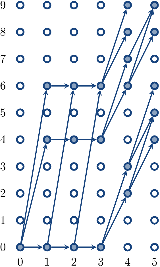
We see that \( \sump(5,4) \) and \( \sump(5,9) \) are true, therefore the constraint is consistent.
Filtering
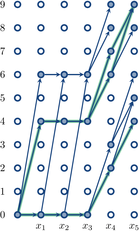
The graph representation shown above allows us to find all the solutions as well: they correspond to the paths from the node \( (0,0) \) to the nodes \( (n,v) \) with \( v \in \Dom{z} \). Namely, if \( (0,0),(1,v_1),…,(n,v_n) \) is such a path, then the solution is
\( x_1 = (v_1-0)/c_1 \),
\( x_2 = (v_2-v_1)/c_2 \),
\( x_n = (v_n-v_{n-1})/c_n \)
Filtering is thus also easy:
\( v \in \DomP{z} \) iff \( v \in \Dom{z} \) and there is a path from the node \( (0,0) \) to \( (n,v) \), and
\( v \in \DomP{x_i} \) iff there is a path \( (0,0),(1,v_1),…,(n,v_n) \) such that \( v_n \in \Dom{z} \) and \( x_i = (v_i-v_{i-1})/c_i \).
Finding all the edges that take part in some of the paths above is easy: just follow the edges backwards from the nodes \( (n,v) \) with \( v \in \Dom{z} \).
Example
Consider again the sum constraint $$2 x_1 + 2 x_2 + 2 x_3 + x_4 + x_5 = z$$ under the domains \( \Dom{x_1} = \Set{0,2,3} \), \( \Dom{x_2} = \Set{0,3} \), \( \Dom{x_3} = \Set{0,3} \), \( \Dom{x_4} = \Set{2,3} \), \( \Dom{x_5} = \Set{2,3} \), and \( \Dom{z} = \Set{4,7,9} \). From the highlighted edges we see that the constraint has three solutions:
\( x_1=0,x_2=0,x_3=0,x_4=2,x_5=2 \)
\( x_1=2,x_2=0,x_3=0,x_4=2,x_5=2 \), and
\( x_1=2,x_2=0,x_3=0,x_4=3,x_5=3 \).
We can thus reduce the domains to \( \Dom{x_1} = \Set{0,2} \), \( \Dom{x_2} = \Set{0} \), \( \Dom{x_3} = \Set{0} \), \( \Dom{x_4} = \Set{2,3} \), \( \Dom{x_5} = \Set{2,3} \), and \( \Dom{z} = \Set{4,9} \).
When implemented with arrays, the dynamic programming approach only works well if the constants and domain values are reasonably small. When implemented with dynamic sets, the approach works well if the number of possible values of \( \sum_{j=1}^i c_jx_j \) for each \( i \) is manageable. For the other cases (large domains etc), one can use weaker filtering that does not enforce arc-consistency. For instance, for each \( i \) one can compute the sum \( m_i = \sum_{j \in \Set{1,…,i-1,i+1,…,n}} c_j \min \Dom{x_j} \) and remove the values \( v \) from \( \Dom{x_i} \) for which \( m_i + c_i v > \max \Dom{z} \).
The all-different constraint
Recall that an all-different global constraint $$\AllDiff{\CVarI 1,…,\CVarI n}$$ requires that the values assigned to the variables \( \CVarI 1,…,\CVarI n \) are pairwise distinct. We now show a graph theoretical way for consistency checking and filtering of all-different constraints.
Consistency checking
We can reduce the consistency problem of \( \AllDiffC \) constraints to the matching problem in unweighted bipartite graphs [vanHoeveKatriel2006]. As there are efficient algorithms for solving the matching problem, the consistency problem can be solved efficiently as well.
Mathematically, an unweighted bipartite graph is a triple \( \Tuple{U,W,E} \), where
\( U \) and \( W \) are two disjoint, finite and non-empty sets of vertices, and
\( E \subseteq {U \times W} \) is a set of edges.
A matching in such a graph is a subset \( M \subseteq E \) of the edges such that for all disjoint edges \( \Tuple{u_1,w_1},\Tuple{u_2,w_2} \in M \) it holds that \( u_1 \neq u_2 \) and \( w_1 \neq w_2 \). In other words, a matching associates each vertex with at most one edge. A matching \( M \) covers a vertex \( u \in U \) if \( \Tuple{u,w} \in M \) for some \( w \in W \).
Example
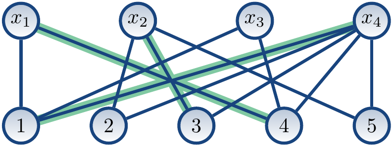
The bipartite graph \( \Tuple{U,W,E} \) with \begin{array}{rcl} U &=& \Set{x_1,x_2,x_3,x_4}\\\\ W &=& \Set{1,2,3,4,5}\\\\ E &=& \{\Tuple{x_1,1},\Tuple{x_1,4},\Tuple{x_2,2},\Tuple{x_2,3},\Tuple{x_2,5},\Tuple{x_3,1},\Tuple{x_3,4},\\\\ & & \ \Tuple{x_4,1},\Tuple{x_4,2},\Tuple{x_4,3},\Tuple{x_4,4},\Tuple{x_4,5}\} \end{array} is shown below. The matching \( \Set{\Tuple{x_1,4},\Tuple{x_2,3},\Tuple{x_4,1}} \) is shown with the highlighted edges. It covers the vertices \( x_1 \), \( x_2 \) and \( x_4 \) but not the vertex \( x_3 \).
The reduction from \( \AllDiffC \) constraints to undirected bipartite graphs is rather simple:
Definition: Value graphs
Assume an all-different constraint \( \AllDiff{\CVarI 1,…,\CVarI k} \) and some domains \( \Dom{\CVarI 1} \),…,\( \Dom{\CVarI k} \). The value graph of the constraint under the domains is the undirected bipartite graph \( \Tuple{\Set{\CVarI 1,…,\CVarI k},\bigcup_{i=1}^k\Dom{\CVarI i},E} \), where \( E = \Setdef{\Tuple{\CVarI i,v}}{1 \le i \le k \land v \in \Dom{\CVarI i}} \).
The vertices in \( \Set{\CVarI 1,…,\CVarI k} \) are called variable vertices and the ones in \( \bigcup_{i=1}^k\Dom{\CVarI i} \) value vertices.
Example
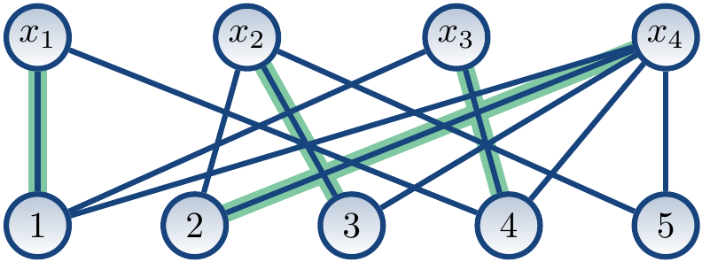
The value graph of the constraint \( \AllDiff{x_1,x_2,x_3,x_4} \) under the domains \( \Dom{x_1} = \Set{1,4} \), \( \Dom{x_2} = \Set{2,3,5} \), \( \Dom{x_3} = \Set{1,4} \), and \( \Dom{x_4} = \Set{1,2,3,4,5} \) is shown below.
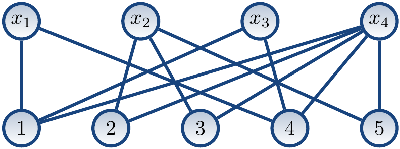
By construction, each solution to the constraint corresponds to a matching that covers all the variable vertices of the value graph. Conversely, each matching that covers all the variable vertices of the value graph corresponds to a solution to the constraint. Therefore, the constraint is consistent if the value graph has a matching that covers all the variable vertices.
Example
Consider again the constraint \( \AllDiff{x_1,x_2,x_3,x_4} \) and the domains \( \Dom{x_1} = \Set{1,4} \), \( \Dom{x_2} = \Set{2,3,5} \), \( \Dom{x_3} = \Set{1,4} \), and \( \Dom{x_4} = \Set{1,2,3,4,5} \).
The matching corresponding to the solution \( \Set{x_1 \mapsto 1,x_2 \mapsto 3,x_3 \mapsto 4,x_4 \mapsto 2} \) is shown below with highlighted edges.
Whether a value graph has a matching covering all variable vertices can be found by computing a maximum matching, a matching having largest possible number of edges, for the graph and checking whether it covers all the variable vertices. A maximum matching can be found, e.g., with the Hopcroft-Karp algorithm. A simplified version of this algorithm is presented next.
Assume a bipartite graph \( G = \Tuple{U,W,E} \) and a matching \( M \subseteq E \). We say that a vertex is \( M \)-free if it does not occur in any edge in \( M \). An augmenting path for \( M \) is a path in \( G \) that starts and ends in an \( M \)-free vertex and alternates between edges not in \( M \) and in \( M \). The following two facts on augmenting paths allow us to find a maximum matching:
A matching is maximum if there are no augmenting paths for it.
If \( M \) has an augmenting path \( p \), a larger matching can be obtained by taking the symmetric difference of \( M \) and the edges in \( p \).
Based on this, we obtain an algorithm for finding a maximum matching:
Start with an empty matching \( M \)
Search for an augmenting path \( p \)
If none is found, return \( M \)
Otherwise, assign \( M \) to the symmetric difference of \( M \) and the edges in \( p \) and repeat
Augmenting paths can be easily found with breadth-first search.
Example: Finding a maximum matching
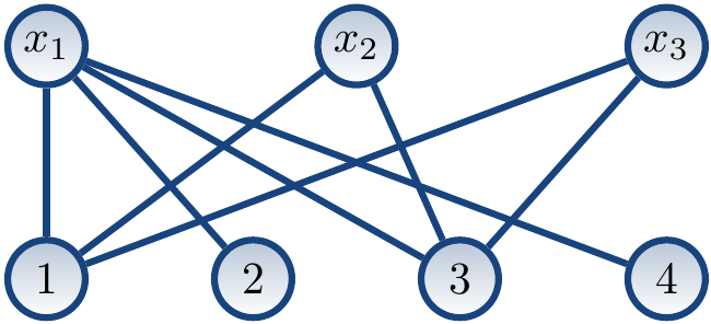
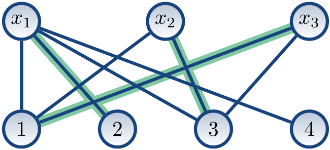
The value graph for the constraint \( \AllDiff{x_1,x_2,x_3} \) with the domains \( \Dom{x_1}=\Set{1,2,3,4} \), \( \Dom{x_2}=\Set{1,3} \), and \( \Dom{x_3}=\Set{1,3} \) is shown below.
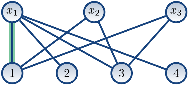
We start with the empty matching \( M = \emptyset \). We may first find the augmenting path \( \Seq{x_1,1} \). After this, the matching is \( M = \Set{\Tuple{x_1,1}} \), shown below with highlighted edges.
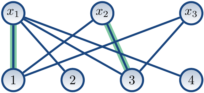
The next the augmenting path could be \( \Seq{x_2,3} \). After this, the matching is \( M = \Set{\Tuple{x_1,1},\Tuple{x_2,3}} \):
The next the augmenting path could be \( \Seq{x_3,1,x_1,2} \), giving the matching \( M = \Set{\Tuple{x_1,2},\Tuple{x_2,3},\Tuple{x_3,1}} \):
The are no more augmenting paths. All variable vertices are covered and a solution is \( \Set{x_1 \mapsto 2, x_2 \mapsto 3, x_3 \mapsto 1} \).
Filtering
By using value graphs, all-different constraints can be filtered to arc-consistency in polynomial time. As stated earlier,
each solution to the constraint corresponds to a value vertex covering matching of the value graph, and
each value vertex covering matching of the value graph corresponds to a solution to the constraint.
Thus if an edge \( \Tuple{\Var,\Val} \) in the value graph does not appear in any value vertex covering matching, the element \( \Val \) can be removed from the domain \( \Dom \Var \).
Once one maximum matching is found, we can find all edges that appear in some maximum matching [Tassa2012] [vanHoeveKatriel2006]. Assume a bipartite graph \( G = \Tuple{U,W,E} \) and a maximum matching \( M \subseteq E \). Build the directed graph \( G_M = \Tuple{U \cup W, \Setdef{\Tuple{u’,w’}}{\Tuple{u’,w’} \in M} \cup \Setdef{\Tuple{w’,u’}}{\Tuple{u’,w’} \in E \setminus M}} \). Now an edge \( \Tuple{u,w} \) belongs to some maximum matching if
\( \Tuple{u,w} \in M \),
\( \Tuple{u,w} \) is an edge inside a strongly connected component of \( G_M \), or
\( \Tuple{u,w} \) appears in a path of \( G_M \) that starts from an \( M \)-free vertex
Strongly connected components can be computed efficiently with Tarjan’s algorithm or with Kosaraju’s algorithm.
Example
Consider again our running example having the value graph \( G \) and a maximum matching \( M \) shown below.
The directed graph \( G_M \) is the following.
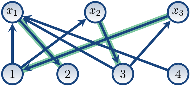
Now:
The edges \( \Tuple{x_1,2} \), \( \Tuple{x_2,3} \) and \( \Tuple{x_3,1} \) in \( M \) belong to some maximum matching.
The directed graph has only one non-singleton strongly connected component, \( \Set{x_2,3,x_3,1} \). Thus the edges \( \Tuple{x_2,1} \) and \( \Tuple{x_3,3} \) belong to some maximum matching.
As \( \Seq{4,x_1} \) is a path of the form required by the third case, \( \Tuple{x_1,4} \) belongs to some maximum matching.
The edge \( \Tuple{x_1,1} \) cannot be included with any one three cases above. Therefore, the value \( 1 \) can be removed from the domain of \( x_1 \). The same applies to edge \( \Tuple{x_1,3} \) and thus the value \( 3 \) can be removed from the domain of \( x_1 \).
Indeed, the constraint has the four solutions \( \Set{x_1 \mapsto 2, x_2 \mapsto 1, x_3 \mapsto 3} \), \( \Set{x_1 \mapsto 4, x_2 \mapsto 1, x_3 \mapsto 3} \), \( \Set{x_1 \mapsto 2, x_2 \mapsto 3, x_3 \mapsto 1} \), and \( \Set{x_1 \mapsto 4, x_2 \mapsto 3, x_3 \mapsto 1} \).