Backtracking Search¶

How can we solve CSP instances? That is, how can we deduce whether a set of constraints is satisfiable or not, or to find an optimal solution for them? When the domains are finite, CSP instances could be solved by

reducing the CSP instance to a SAT instance, and then
solving the SAT instance with a SAT solver.

Indeed, some CSP solvers do this. However, performing a backtracking search and constraint propagation on the global constraints level can result in better performance as

the expansion of non-binary domains and global constraints to the Boolean level can be quite large, and
one can use efficient custom algorithms for propagating global constraints.

Below is a very simple backtracking search procedure that

first performs constraint propagation, and
if the solution is not yet found, selects a variable and then recursively searches for a solution in which the variable has a fixed value from its domain.

def \( \PseudoSolve(\Constrs,\DomF) \):
    \( \DomPF \PseudoAsgn \PseudoPropagate(\Constrs,\DomF) \)
    if \( \Constrs \) has a constraint \( \Constr \) that is inconsistent under \( \DomPF \): return \( \PseudoUnsat \)
    if \( \Card{\DomP{x}} = 1 \) for all the variables \( x \): return \( \PseudoSat \)
    choose a variable \( x \) with \( \DomP{x} = \Set{v_1,...,v_k} \) and \( k \ge 2 \)
    for each \( v \in \Set{v_1,...,v_k} \):
        \( r \PseudoAsgn \PseudoSolve(\Constrs,\FixD{\DomPF}{x}{\Set{v}}) \)
        if \( r = \PseudoSat \): return \( \PseudoSat \)
    return \( \PseudoUnsat \)
 

Example

Consider a simple ARM architecture assembly program with symbolic register names below.

  LDR a, a_addr  // a_addr is the address of the input array
  MOV i, #0      // i = 0
  MOV s, #0      // s = 0
loop:
  CMP i, #10            // if i >= 10, goto end
  BGE end
  LDR t, [a, i, LSL#2]  // t = a[i]
  MUL v, t, t           // v = t * t
  ADD s, s, v           // s = s + v
  ADD i, i, #1          // i = i + 1
  B   loop
end:
  LDR b, b_addr  // save s to the memory location b_addr
  STR s, [b]

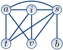
If we perform a liveness analysis for the registers, we get a register-inference graph (see e.g. Aho, Sethi, and Ullman: “Compilers: Principles, Techniques, and Tools”) shown below. It has an edge between register nodes if and only if there is a line in which one register is written to and the other can be read later without being written to in between. The graph is $ k $-colorable iff the program can be implemented by using only $ k $ hardware registers and no spills to the memory.

The graph $ k $-coloring problem can be easily expressed as a CSP problem by taking a variable for each vertex. The domain of all the variables is a set of $ k $ colors. The constraints are $ x \neq y $ for each edge between $ x $ and $ y $ in the graph. 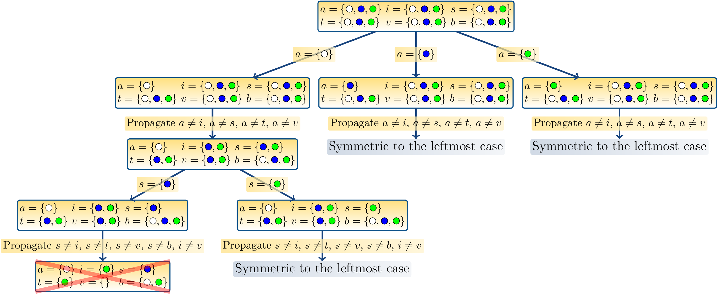In our simple example, the constraints are $$\begin{array}{lll} a \neq i & a \neq s & a \neq t & a \neq v & i \neq s \\\\ i \neq t & i \neq v & s \neq t & s \neq v & s \neq b & \end{array}$$ A search tree for our instance when three colors are allowed is shown below. Each node describes the domains either when entering the solve call or after constraint propagation.

The instance has no solutions as all the branches end in a situation where the domain of some variable is empty.

Our example graph is colorable with 4 colors and thus the program can be implemented with 4 registers:

  LDR R0, a_addr  // a_addr is the address of the input array
  MOV R1, #0      // i = 0
  MOV R2, #0      // s = 0
loop:
  CMP R1, #10              // if i >= 10, goto end
  BGE end
  LDR R3, [R0, R1, LSL#2]  // t = a[i]
  MUL R3, R3, R3           // v = t * t
  ADD R2, R2, R3           // s = s + v
  ADD R1, R1, #1           // i = i + 1
  B   loop
end:
  LDR R3, b_addr  // save s to the memory location b_addr
  STR R2, [R3]

The above description of the backtracking search scheme is simplified and omits many details. For instance, the variable selection heuristic, i.e. how one chooses the variable $ x $ whose domain $ \Set{v_1,…,v_k} $ is split into $ \Set{v_1} $,…,$ \Set{v_k} $, is very important but not discussed further in this course. And one could also split the domain $ \Set{v_1,…,v_k} $ of the branching variable $ x $ differently, for instance into $ \Set{v_1,…,v_{k/2}} $ and $ \Set{v_{k/2+1},…,v_k} $ if $ k $ is large. Some solvers allow the user to control these aspects and thus tune the solver for specific problem types.