Global constraints
A global constraint is a “constraint that captures a relation between a non-fixed number of variables” [vanHoeveKatriel2006]. For instance, an “all-different” global constraint $$\AllDiff{\CVarI 1,…,\CVarI n}$$ requires that the values assigned to the variables \( \CVarI 1,…,\CVarI n \) are pairwise distinct. In many cases, global constraints are semantically redundant as they can be expressed with some simpler constraints. For instance, \( \AllDiff{\CVarI 1,…,\CVarI n} \) could be expressed with \( \frac{n(n-1)}{2} \) disequalities $$\bigwedge_{1 \le i < j \le n} (\CVarI i \neq \CVarI j)$$ In fact, some solvers transform all-different constraints to this form internally. However, having higher-level shorthands like \( \AllDiff{\CVarI 1,…,\CVarI n} \)
makes the problem description task easier as, for instance, the user does not have to write \( \frac{n(n-1)}{2} \) binary disequalities but only one \( \AllDiffC \) constraint with \( n \) arguments, and
allows the constraint solver to have a higher-level view of the structure of the problem and potentially use better constraint propagation techniques.
Hundreds of global constraints have been defined, see, for instance, the global constraints catalog. In the following, we
introduce a few commonly used global constraints, and
next describe how some of them can be solved and propagated algorithmically.
The all-different global constaint
As our first global constraint, let us study the all-different constraint.
A constraint \( \AllDiff{\CVarI1,…,\CVarI{n}} \) requires that the values assigned to the variables \( \CVarI1,…,\CVarI{n} \) are mutually distinct.
Formally, \( \AllDiff{\CVarI1,…,\CVarI{n}} \) corresponds to the set
$$\Setdef{(v_1,…,v_n) \in \Dom{\CVarI1}\times … \times \Dom{\CVarI{n}}}{v_i \neq v_j \textrm{ for all } 1 \le i < j \le n}$$
of tuples.
As an application example, let’s see how Sudokus can be modelled and solved
with the MiniZinc language.
The “model” file, call it sudoku.mzn,
describes the variable types and the constraints:
% Import all-different global constraint
include "alldifferent.mzn";
% Sub-grid dimension constant, from an external data file
int: D;
% Grid dimension, a constant as well
int: N = D * D;
% A 2-dimensional array for the solution
array [1..N,1..N] of var 1..N: grid;
% The input clues, from an external data file, 0 means empty cell
array [1..N,1..N] of 0..N: clues;
% The solution should respect the clues
constraint forall (row in 1..N, col in 1..N) (
  clues[row,col] > 0 -> grid[row,col] == clues[row,col]);
% The values in each row should be distinct
constraint forall (row in 1..N) (alldifferent([grid[row,col] | col in 1..N]));
% The values in each column should be distinct
constraint forall (col in 1..N) (alldifferent([grid[row,col] | row in 1..N]));
% The values in each distinct sub-grid should be distinct
constraint forall (subrow, subcol in 1..D)(
  alldifferent([grid[(subrow-1) * D + rowd, (subcol-1) * D + cold] | rowd,cold in 1..D]));
% Solve the problem
solve satisfy;
% Solution output
int: digits = ceil(log(10.0,int2float(N)));
output [ show_int(digits,grid[row,col]) ++ " " ++ if col mod D == 0 then " " else "" endif ++
  if col == N /\ row != N then if row mod D == 0 then "\n\n" else "\n" endif else "" endif
  | row,col in 1..N ] ++ ["\n"];
In MiniZinc, the problem instance data can be given in a separate “data” file
so that the same model can be used for different instances.
For the previous sudoku model we could have
the data file sudoku-royle.dzn:
D = 3;
clues = [|
0,0,0,0,0,0,0,1,0|
4,0,0,0,0,0,0,0,0|
0,2,0,0,0,0,0,0,0|
0,0,0,0,5,0,4,0,7|
0,0,8,0,0,0,3,0,0|
0,0,1,0,9,0,0,0,0|
3,0,0,4,0,0,2,0,0|
0,5,0,1,0,0,0,0,0|
0,0,0,8,0,6,0,0,0|];
The corresponding sudoku puzzle, taken from Gordon Royle’s minimum Sudoku collection, is:
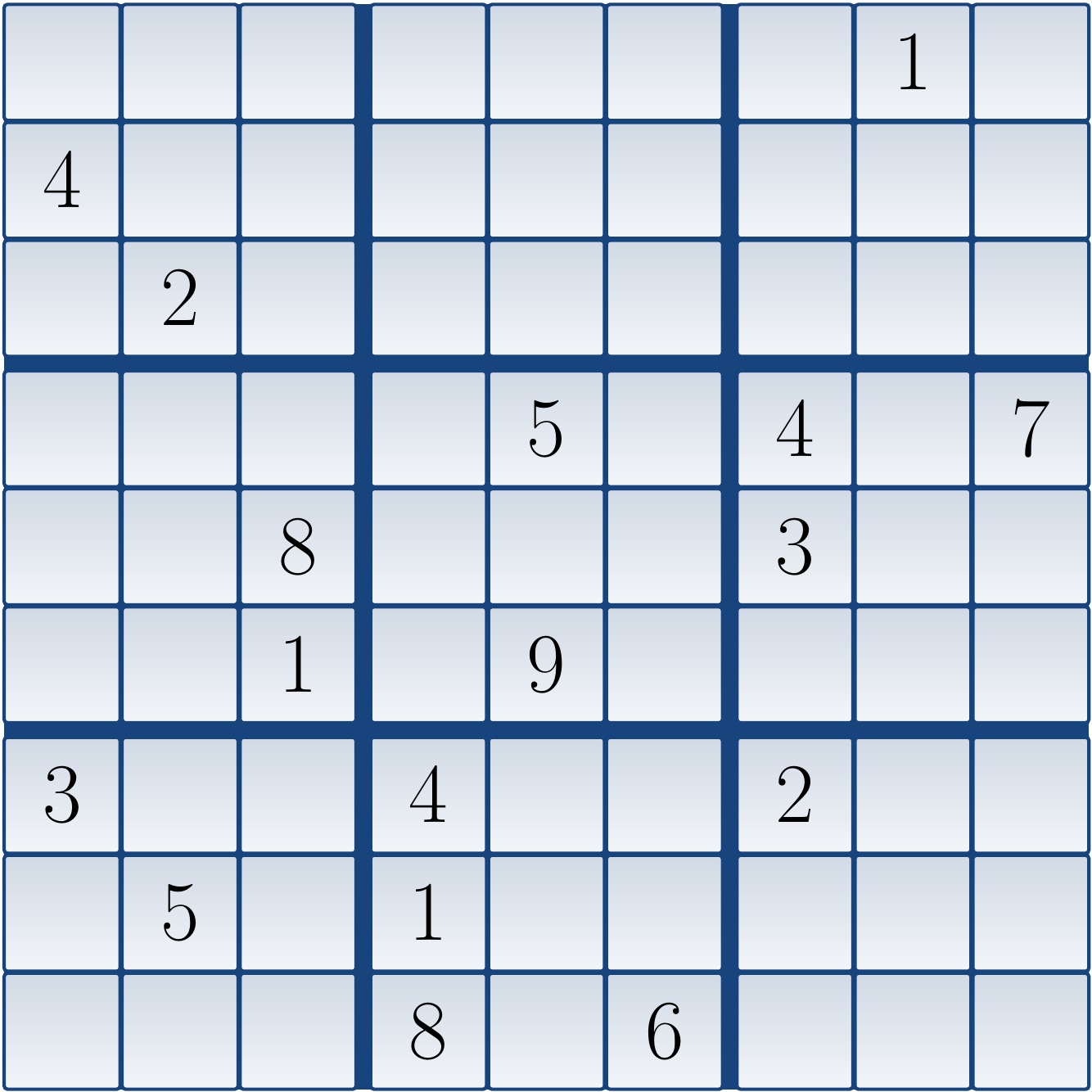
Solving the model and data file with the gecode solver, which is bundled in the MiniZinc distribution, produces a solution for the sudoku grid:
cs-167 % mzn-gecode sudoku.mzn sudoku-royle.dzn
6 9 3  7 8 4  5 1 2
4 8 7  5 1 2  9 3 6
1 2 5  9 6 3  8 7 4

9 3 2  6 5 1  4 8 7
5 6 8  2 4 7  3 9 1
7 4 1  3 9 8  6 2 5

3 1 9  4 7 5  2 6 8
8 5 6  1 2 9  7 4 3
2 7 4  8 3 6  1 5 9
----------
The sum global constraint
A very common requirement in many problems is that the values of some integer variables should sum up to some value. This can be captured with the “sum” global constraint $$c_1 y_1 + … + c_n y_n = z,$$ where the \( c_i \)s are integer constants and \( y_1,…,y_n,z \) are integer-valued variables. More formally, such a sum can be seen as the constraint $$\Sum{\CVarI1,…,\CVarI{n}}{\vec{c}}{z}$$ where \( \vec{c} \) is a vector of \( n \) integer constants; this constraint corresponds to the set of tuples $$\Setdef{\Tuple{v_1,…,v_n,w} \in \Dom{\CVarI1}\times…\times\Dom{\CVarI{n}}\times\Dom{z}}{c_1v_1+…+c_nv_n=w}.$$
In MiniZinc, sums over some fixed set of variables can be written
in the usual infix form (recall the “verbal arithmetic” example).
Sums over the values in an array can be computed with the sum construct.
For instance, if \( a \) is an array of \( N \) integers such as
array [1..N] of var 1..K: a;
then the sum of its elements can be expressed with
sum(i in 1..N)(a[i])
Multi-dimensional arrays and filtering are also supported. For instance,
sum(i in 1..N, j in 1..M where b[i,j] >= 4)(b[i,j])
means the sum of all the elements whose value is at least 4 in a 2-dimensional \( N \times M \)-array \( b \).
The cumulative global constraint
In addition to “generic” global constraints such as all-different and sum, several more “application-oriented” global constraints have been introduced and studied. An example is the \( \CumuC \) global constraint that is used for modelling cumulative resourse use of independent tasks. For \( n \) tasks, the constraint $$\Cumu{\Seq{s_1,…,s_n},\Seq{d_1,…,d_n},\Seq{r_1,…,r_n},b}$$ is satisfied if each task \( i \)
is started at time \( s_i \),
runs \( d_i \) time units, and
uses \( r_i \) resourses when running,
and the tasks running at the same time use at most \( b \) resourses at any time point.
Example
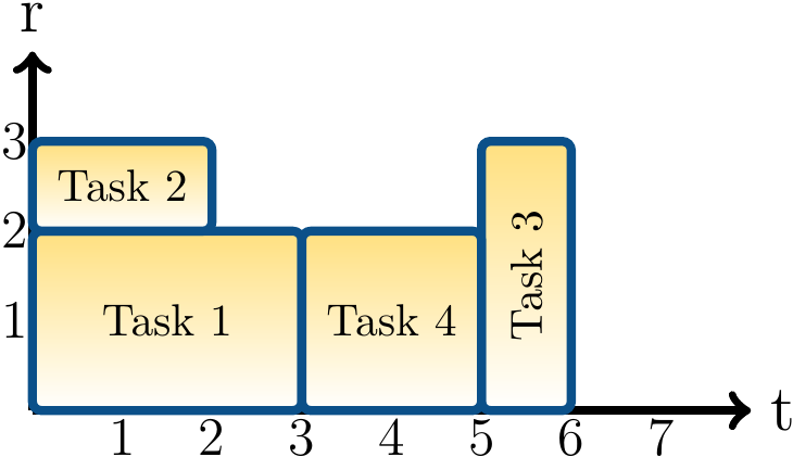
Suppose that we wish to find out the minimum amount of time that is required to run four tasks, \( t_1,…,t_4 \), so that at most 3 resources are used at any moment and
\( t_1 \) runs for 3 units and uses 2 resourses,
\( t_2 \) runs for 2 units and uses 1 resourse,
\( t_3 \) runs for 1 unit and uses 3 resourses, and
\( t_4 \) runs for 2 unit2 and uses 2 resourses.
In MiniZinc, the following model file can be used to find the shortest time in which we can run an arbitrary set of tasks:
% Import the global constraint
include "cumulative.mzn";
% The number of tasks, from an external data file
int: n;
% Indices for tasks, TASKS = {1,2,...,n}
set of int: TASKS = 1..n;
% The durations and resource use of tasks
array[TASKS] of int: dur;        % From an external data file
array[TASKS] of int: resources;  % From an external data file
% The maximum amount of resources available at any time point
int: max_resources;  % From an external data file

% An upper bound for the total time use
int: max_time = sum(t in TASKS)(dur[t]);
% The start times of the tasks
array[TASKS] of var 0..max_time: start;
% The end time of the last task, i.e., the total time use
var 0..max_time: end;
% The tasks should not use more than max_resources resources at any time
constraint cumulative(start, dur, resources, max_resources);
% Force the total time use to have correct value
constraint forall(t in TASKS)(start[t]+dur[t] <= end);
% Optimize: find a solution that minimizes total time use
solve minimize end;
% Output the solution
output ["start=\(start)\n", "end=\(end)\n"];
The following data file then describes the current problem instance:
n = 4;
% The durations of the tasks
dur = [3,2,1,2];
% The resource usages of the tasks
resources = [2,1,3,2];
% The maximum amount of resources available at any time point
max_resources = 3;
Solving this gives us a solution with minimal total time use:
start=[0, 0, 5, 3]
end=6
An illustration of a solution with minimal total time use: