Compute RSA between RDMs

This example showcases the most basic version of RSA: computing the similarity between two RDMs. Then we continue with computing RSA between many RDMs efficiently.

# sphinx_gallery_thumbnail_number=2

import mne
import mne_rsa

# Import required packages
import pandas as pd
from matplotlib import pyplot as plt

MNE-Python contains a build-in data loader for the kiloword dataset, which is used here as an example dataset. Since we only need the words shown during the experiment, which are in the metadata, we can pass preload=False to prevent MNE-Python from loading the EEG data, which is a nice speed gain.

data_path = mne.datasets.kiloword.data_path(verbose=True)
epochs = mne.read_epochs(data_path / "kword_metadata-epo.fif")

# Show the metadata of 10 random epochs
epochs.metadata.sample(10)

	WORD	Concreteness	WordFrequency	OrthographicDistance	NumberOfLetters	BigramFrequency	ConsonantVowelProportion	VisualComplexity
318	error	3.000000	2.564666	2.10	5.0	305.600000	0.600000	54.891308
762	loft	5.400000	1.672098	1.55	4.0	180.750000	0.750000	51.216248
786	grace	2.550000	2.572872	1.40	5.0	633.600000	0.600000	71.031177
105	nature	4.300000	3.525563	1.95	6.0	449.000000	0.500000	62.193324
401	content	3.400000	2.498311	1.70	7.0	1268.714286	0.714286	61.886538
609	cavity	5.400000	1.716003	2.25	6.0	465.666667	0.500000	58.809211
468	syndrome	3.750000	1.968483	3.95	8.0	277.750000	0.625000	71.186959
62	chair	5.850000	3.265054	1.70	5.0	445.600000	0.600000	58.749419
464	heritage	3.150000	2.276462	2.80	8.0	552.750000	0.500000	66.750923
951	colossus	4.578947	1.397940	2.90	8.0	665.375000	0.625000	64.001385

Compute RDMs based on word length and visual complexity.

metadata = epochs.metadata
rdm1 = mne_rsa.compute_rdm(metadata.NumberOfLetters, metric="euclidean")
rdm2 = mne_rsa.compute_rdm(metadata.VisualComplexity, metric="euclidean")

# Plot the RDMs
mne_rsa.plot_rdms([rdm1, rdm2], names=["Word length", "Vis. complexity"])

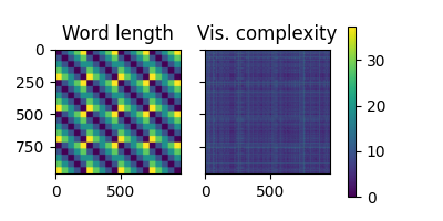
<Figure size 400x200 with 3 Axes>

Perform RSA between the two RDMs using Spearman correlation

rsa_result = mne_rsa.rsa(rdm1, rdm2, metric="spearman")
print("RSA score:", rsa_result)

RSA score: 0.02643988328911863

We can compute RSA between multiple RDMs by passing lists to the mne_rsa.rsa() function.

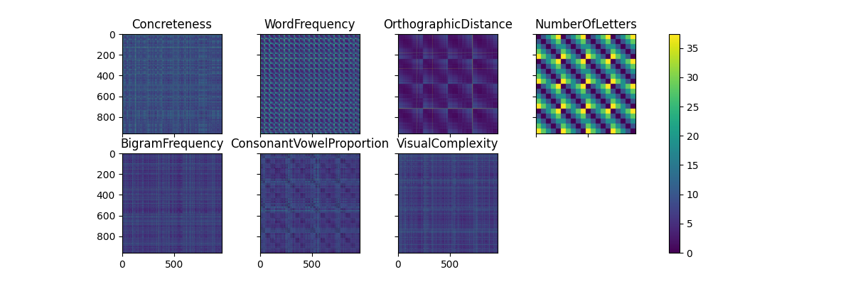
# Create RDMs for each stimulus property
columns = metadata.columns[1:]  # Skip the first column: WORD
rdms = [mne_rsa.compute_rdm(metadata[col], metric="euclidean") for col in columns]

# Plot the RDMs
fig = mne_rsa.plot_rdms(rdms, names=columns, n_rows=2)
fig.set_size_inches(12, 4)

# Compute RSA between the first two RDMs (Concreteness and WordFrequency) and the
# others.
rsa_results = mne_rsa.rsa(rdms[:2], rdms[2:], metric="spearman")

# Pack the result into a Pandas DataFrame for easy viewing
print(pd.DataFrame(rsa_results, index=columns[:2], columns=columns[2:]))

               OrthographicDistance  NumberOfLetters  BigramFrequency  ConsonantVowelProportion  VisualComplexity
Concreteness               0.031064         0.026832        -0.004681                  0.005647          0.004263
WordFrequency              0.058385         0.013607         0.001970                 -0.003850         -0.009620

What if we have many RDMs? The mne_rsa.rsa() function is optimized for the case where the first parameter (the “data” RDMs) is a large list of RDMs and the second parameter (the “model” RDMs) is a smaller list. To save memory, you can also pass generators instead of lists.

Let’s create a generator that creates RDMs for each time-point in the EEG data and compute the RSA between those RDMs and all the “model” RDMs we computed above. This is a basic example of using a “searchlight” and in other examples, you can learn how to use the searchlight generator to build more advanced searchlights. However, since this is such a simple case, it is educational to construct the generator manually.

The RSA computation will take some time. Therefore, we pass a few extra parameters to mne_rsa.rsa() to enable some improvements. First, the verbose=True enables a progress bar. However, since we are using a generator, the progress bar cannot automatically infer how many RDMs there will be. Hence, we provide this information explicitly using the n_data_rdms parameter. Finally, depending on how many CPUs you have on your system, consider increasing the n_jobs parameter to parallelize the computation over multiple CPUs.

epochs.resample(100)  # Downsample to speed things up for this example
eeg_data = epochs.get_data()
n_trials, n_sensors, n_times = eeg_data.shape


def generate_eeg_rdms():
    """Generate RDMs for each time sample."""
    for i in range(n_times):
        yield mne_rsa.compute_rdm(eeg_data[:, :, i], metric="correlation")


rsa_results = mne_rsa.rsa(
    generate_eeg_rdms(),
    rdms,
    metric="spearman",
    verbose=True,
    n_data_rdms=n_times,
    n_jobs=1,
)

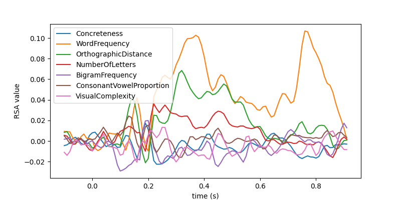
# Plot the RSA values over time using standard matplotlib commands
plt.figure(figsize=(8, 4))
plt.plot(epochs.times, rsa_results)
plt.xlabel("time (s)")
plt.ylabel("RSA value")
plt.legend(columns)

/m/home/home4/45/vanvlm1/data/projects/mne-rsa/examples/plot_rsa_between_rdms.py:89: FutureWarning: The current default of copy=False will change to copy=True in 1.7. Set the value of copy explicitly to avoid this warning
  eeg_data = epochs.get_data()

  0%|          | 0/102 [00:00<?, ?RDM/s]
  1%|          | 1/102 [00:00<00:32,  3.08RDM/s]
  2%|▏         | 2/102 [00:00<00:33,  2.96RDM/s]
  3%|▎         | 3/102 [00:01<00:33,  2.93RDM/s]
  4%|▍         | 4/102 [00:01<00:33,  2.91RDM/s]
  5%|▍         | 5/102 [00:01<00:34,  2.81RDM/s]
  6%|▌         | 6/102 [00:02<00:34,  2.75RDM/s]
  7%|▋         | 7/102 [00:02<00:36,  2.63RDM/s]
  8%|▊         | 8/102 [00:02<00:37,  2.49RDM/s]
  9%|▉         | 9/102 [00:03<00:35,  2.60RDM/s]
 10%|▉         | 10/102 [00:03<00:34,  2.68RDM/s]
 11%|█         | 11/102 [00:04<00:33,  2.74RDM/s]
 12%|█▏        | 12/102 [00:04<00:31,  2.82RDM/s]
 13%|█▎        | 13/102 [00:04<00:31,  2.82RDM/s]
 14%|█▎        | 14/102 [00:05<00:30,  2.85RDM/s]
 15%|█▍        | 15/102 [00:05<00:30,  2.89RDM/s]
 16%|█▌        | 16/102 [00:05<00:29,  2.89RDM/s]
 17%|█▋        | 17/102 [00:06<00:29,  2.93RDM/s]
 18%|█▊        | 18/102 [00:06<00:28,  2.95RDM/s]
 19%|█▊        | 19/102 [00:06<00:27,  2.97RDM/s]
 20%|█▉        | 20/102 [00:07<00:28,  2.89RDM/s]
 21%|██        | 21/102 [00:07<00:27,  2.92RDM/s]
 22%|██▏       | 22/102 [00:07<00:27,  2.93RDM/s]
 23%|██▎       | 23/102 [00:08<00:26,  2.96RDM/s]
 24%|██▎       | 24/102 [00:08<00:26,  2.98RDM/s]
 25%|██▍       | 25/102 [00:08<00:25,  2.98RDM/s]
 25%|██▌       | 26/102 [00:09<00:25,  3.00RDM/s]
 26%|██▋       | 27/102 [00:09<00:24,  3.01RDM/s]
 27%|██▋       | 28/102 [00:09<00:24,  2.98RDM/s]
 28%|██▊       | 29/102 [00:10<00:24,  3.00RDM/s]
 29%|██▉       | 30/102 [00:10<00:23,  3.02RDM/s]
 30%|███       | 31/102 [00:10<00:23,  3.00RDM/s]
 31%|███▏      | 32/102 [00:11<00:23,  3.01RDM/s]
 32%|███▏      | 33/102 [00:11<00:22,  3.02RDM/s]
 33%|███▎      | 34/102 [00:11<00:22,  2.98RDM/s]
 34%|███▍      | 35/102 [00:12<00:22,  2.99RDM/s]
 35%|███▌      | 36/102 [00:12<00:21,  3.01RDM/s]
 36%|███▋      | 37/102 [00:12<00:21,  3.00RDM/s]
 37%|███▋      | 38/102 [00:13<00:21,  3.01RDM/s]
 38%|███▊      | 39/102 [00:13<00:20,  3.01RDM/s]
 39%|███▉      | 40/102 [00:13<00:21,  2.86RDM/s]
 40%|████      | 41/102 [00:14<00:21,  2.84RDM/s]
 41%|████      | 42/102 [00:14<00:20,  2.87RDM/s]
 42%|████▏     | 43/102 [00:14<00:20,  2.91RDM/s]
 43%|████▎     | 44/102 [00:15<00:19,  2.94RDM/s]
 44%|████▍     | 45/102 [00:15<00:19,  2.95RDM/s]
 45%|████▌     | 46/102 [00:15<00:18,  2.96RDM/s]
 46%|████▌     | 47/102 [00:16<00:18,  2.99RDM/s]
 47%|████▋     | 48/102 [00:16<00:18,  2.98RDM/s]
 48%|████▊     | 49/102 [00:16<00:17,  3.00RDM/s]
 49%|████▉     | 50/102 [00:17<00:17,  3.01RDM/s]
 50%|█████     | 51/102 [00:17<00:16,  3.01RDM/s]
 51%|█████     | 52/102 [00:17<00:16,  3.01RDM/s]
 52%|█████▏    | 53/102 [00:18<00:16,  3.00RDM/s]
 53%|█████▎    | 54/102 [00:18<00:15,  3.01RDM/s]
 54%|█████▍    | 55/102 [00:18<00:15,  3.01RDM/s]
 55%|█████▍    | 56/102 [00:19<00:15,  3.02RDM/s]
 56%|█████▌    | 57/102 [00:19<00:14,  3.02RDM/s]
 57%|█████▋    | 58/102 [00:19<00:14,  3.02RDM/s]
 58%|█████▊    | 59/102 [00:20<00:14,  3.03RDM/s]
 59%|█████▉    | 60/102 [00:20<00:13,  3.03RDM/s]
 60%|█████▉    | 61/102 [00:20<00:13,  3.03RDM/s]
 61%|██████    | 62/102 [00:21<00:13,  3.04RDM/s]
 62%|██████▏   | 63/102 [00:21<00:12,  3.04RDM/s]
 63%|██████▎   | 64/102 [00:21<00:12,  3.04RDM/s]
 64%|██████▎   | 65/102 [00:22<00:12,  3.03RDM/s]
 65%|██████▍   | 66/102 [00:22<00:11,  3.03RDM/s]
 66%|██████▌   | 67/102 [00:22<00:11,  3.02RDM/s]
 67%|██████▋   | 68/102 [00:23<00:11,  3.03RDM/s]
 68%|██████▊   | 69/102 [00:23<00:10,  3.03RDM/s]
 69%|██████▊   | 70/102 [00:23<00:10,  3.02RDM/s]
 70%|██████▉   | 71/102 [00:24<00:10,  3.03RDM/s]
 71%|███████   | 72/102 [00:24<00:09,  3.04RDM/s]
 72%|███████▏  | 73/102 [00:24<00:09,  3.04RDM/s]
 73%|███████▎  | 74/102 [00:25<00:09,  3.05RDM/s]
 74%|███████▎  | 75/102 [00:25<00:08,  3.05RDM/s]
 75%|███████▍  | 76/102 [00:25<00:08,  3.04RDM/s]
 75%|███████▌  | 77/102 [00:26<00:08,  3.03RDM/s]
 76%|███████▋  | 78/102 [00:26<00:07,  3.04RDM/s]
 77%|███████▋  | 79/102 [00:26<00:07,  3.03RDM/s]
 78%|███████▊  | 80/102 [00:27<00:07,  3.03RDM/s]
 79%|███████▉  | 81/102 [00:27<00:06,  3.04RDM/s]
 80%|████████  | 82/102 [00:27<00:06,  3.03RDM/s]
 81%|████████▏ | 83/102 [00:28<00:06,  3.04RDM/s]
 82%|████████▏ | 84/102 [00:28<00:05,  3.04RDM/s]
 83%|████████▎ | 85/102 [00:28<00:05,  3.02RDM/s]
 84%|████████▍ | 86/102 [00:29<00:05,  3.03RDM/s]
 85%|████████▌ | 87/102 [00:29<00:04,  3.04RDM/s]
 86%|████████▋ | 88/102 [00:29<00:04,  3.02RDM/s]
 87%|████████▋ | 89/102 [00:30<00:04,  3.01RDM/s]
 88%|████████▊ | 90/102 [00:30<00:03,  3.02RDM/s]
 89%|████████▉ | 91/102 [00:30<00:03,  3.00RDM/s]
 90%|█████████ | 92/102 [00:31<00:03,  2.99RDM/s]
 91%|█████████ | 93/102 [00:31<00:02,  3.01RDM/s]
 92%|█████████▏| 94/102 [00:31<00:02,  3.01RDM/s]
 93%|█████████▎| 95/102 [00:32<00:02,  3.02RDM/s]
 94%|█████████▍| 96/102 [00:32<00:01,  3.04RDM/s]
 95%|█████████▌| 97/102 [00:32<00:01,  3.00RDM/s]
 96%|█████████▌| 98/102 [00:33<00:01,  3.02RDM/s]
 97%|█████████▋| 99/102 [00:33<00:00,  3.03RDM/s]
 98%|█████████▊| 100/102 [00:33<00:00,  3.02RDM/s]
 99%|█████████▉| 101/102 [00:34<00:00,  3.03RDM/s]
100%|██████████| 102/102 [00:34<00:00,  3.04RDM/s]
100%|██████████| 102/102 [00:34<00:00,  2.97RDM/s]

<matplotlib.legend.Legend object at 0x7fe3836a3190>