Some Theories and Logics¶

In the following, we will introduce some of the most commonly applied theories.

Integer and Real Arithmetic¶

In the general non-linear case, these theories allow inequalities between polynomials. We consider two version,

the theory of non-linear integer arithmetic $ \TNIA $, and
the theory of non-linear real arithmetic $ \TNRA $.

In both versions, the signature consists of the sort, $ \IntsSort $ or $ \RealsSort $, and

the constants $ 0 $ and $ 1 $,
the binary functions $ + $, $ - $, and $ \Mul $, as well as
the binary predicates $ < $ and $ \Eq $.

The other numerals are abbreviations, e.g., $ 5 $ means $ 1+1+1+1+1 $. Likewise for the usual inequalities and constant exponents, e.g., $ x^2 \ge y $ abbreviates $ ({y \Eq x \Mul x} \lor {y < x \Mul x}) $. Instead of axiomatic definitions for these theories, we usually use intended interpretations:

For integers, the domain is $ \Ints $, and $ 0 $, $ 1 $, $ + $, $ - $, $ \Mul $, and $ < $ are interpreted as usual.
For reals, the domain is $ \Reals $, and $ 0 $, $ 1 $, $ + $, $ - $, $ \Mul $, and $ < $ are interpreted as usual. It would actually be enough to use the real algebraic numbers subset as the domain because these numbers are enough for polynomials. Such numbers are computable.

Example

The quantifier-free formula $$(y^2 < 4) \land (x \Neq 0) \land (2 \Mul x \Eq y)$$ is satisfiable over reals but nor over integers.

Example

Rational constants can be expressed as well; for instance, the quantifier-free formula $$a \lor ((x-0.5)^2 \le 0.1)$$ is equivalent to $ a \lor (x*x-x+0.25 \le 0.1) $, i.e., $ a \lor (20*x*x-20*x+5 \le 2) $.

Satisfiability and quantifier-free satisfiability for nonlinear arithmetic over integers are undecidable as Hilbert’s tenth problem is undecidable (also see B. Poonen, Undecidability in Number Theory, Notices of the AMS 33(5):344–350, 2008). As a curiosity, we don’t know whether $ x^3+y^3+z^3=114 $ has an integer solution. A solution for $ x^3+y^3+z^3=30 $, namely $ x=-283059965 $, $ y = -2218888517 $, and $ z = 2220422932 $, as well as to similar equations with some other right hand side values can be found in

M. Beck, E. Pine, W. Tarrant and K. Y. Jensen: New integer representations as the sum of three cubes, Mathematics of Computation 76:1683–1690, 2007

The case $ x^3+y^3+z^3=33 $ was open for a quite long time but solved recently in A. R. Booker: Cracking the problem with 33, 2019.

Satisfiability for nonlinear arithmetic over reals is a decidable problem as it can be solved with the cylindrical algebraic decomposition method.

Linear Arithmetic¶

In many applications, the full non-linear arithmetic is not needed but linear inequalities are enough. The theories of linear arithmetic,

$ \LIA $, Linear Integer Arithmetic, and
$ \LRA $, Linear Real Arithmetic

are thus defined by having the signature consisting of the sort, $ \IntsSort $ or $ \RealsSort $, and

the constants $ 0 $ and $ 1 $,
the binary functions $ + $ and $ - $, as well as
the binary predicates $ < $ and $ \Eq $.

Notice that multiplication is missing so higher-degree polynomials cannot be expressed. However, multiplication by constant is still expressible as, for instance, $ 3x $ is equal to $ x + x + x $. The theory $ \LIA $ has only one structure associating the sort to $ \Ints $ and interpreting the constants, functions, and predicates in the usual way. Similarly for the theory $ \LRA $ (although for linear arithmetic, rationals would suffice as the domain).

For both theories, satisfiability is decidable.

The atoms are usually written in a standard form $$c_1 x_1 + … + c_n x_n \bowtie d$$ where $ c_1,…,c_n,d $ are rational constants and $ {\bowtie} \in \Set{<,\le,\Eq,\ge,>} $. Note that rational constants can be expressed with integers, e.g., $ \frac{3}{5}x - \frac{2}{3}y < 7 $ is equal to $ 9x - 10y < 105 $.

Example

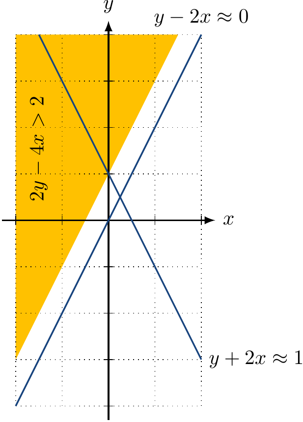
The linear arithmetic formula $$(y - 2x \Eq 0) \land ({y + 2x \Eq 1} \lor {2y - 4x > 2})$$ is

$ \LRA $-satisfiable ($ x = 0.25, y=0.5 $) but
$ \LIA $-unsatisfiable.

Note

Axiomatic definitions of arithmetic are also possible but they are more complex, have non-standard models, or are incomplete in first-order logic (need second-order logic). For instance, (unsorted) Presburger arithmetic for natural numbers with addition has

the signature with constants $ 0 $ and $ 1 $, and the binary function $ + $, and
the axioms
- $ \Forall{x}{\neg(x+1 \Eq 0)} $
- $ \Forall{x,y}{x + 1 \Eq y + 1 \Implies x \Eq y} $
- $ \Forall{x}{x + 0 \Eq x} $
- $ \Forall{x,y}{x + (y + 1) \Eq (x + y) + 1} $
- $ (P(0) \land \Forall{x}{(P(x) \Rightarrow P(x + 1))}) \Implies \Forall{y}{P(y)} $ for each first-order formula $ P(x) $ in the language of Presburger arithmetic with a free variable $ x $ (and possibly other free variables). This is an axiom schema instantiating into countably many axioms.

Similarly, see Peano arithmetic for natural numbers with addition and multiplication and Tarski’s axiomatization of the real numbers.

Difference Logic¶

Difference logic is a further syntactic restriction of linear arithmetic, where the atoms are required to be of the form \[x_1 - x_2 \bowtie c\] (or equivalently $ x_1 \bowtie x_2 + c $), where $ x_1 $ and $ x_2 $ are variables, $ {\bowtie} \in \Set{<,\le,\Eq,\ge,>} $, and $ c \in \Rats $ is a rational constant. That is, the atoms can only constrain the difference between $ x_1 $ and $ x_2 $. With a simple trick, atoms of form $ x \bowtie c $ can be allowed as well. Again, we have integer- and real-valued versions:

$ \RDL $, Real Difference Logic, and
$ \IDL $, Integer Difference Logic.

Example

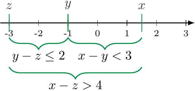
The formula $$(x < y + 3) \land (y \le z+2) \land (z < x - 4)$$ is $ \RDL $-satisfiable (e.g., the interpretation $ \Set{x \mapsto 1.5, y \mapsto -1, z \mapsto -3} $ evaluates it to true) but $ \IDL $-unsatisfiable.

Example: Jobshop scheduling with difference logic

Consider the following problem. We are given a finite set of jobs of the form $$\JSJob{j} = \List{\JSTask{j}{1}=\Tuple{\JSMach{j}{1},\JSDur{j}{1}},…,\JSTask{j}{\JSNofTasks{j}}=\Tuple{\JSMach{j}{\JSNofTasks{1}},\JSDur{j}{\JSNofTasks{j}}}}$$ where each task $ \JSTask{j}{i} = \Tuple{\JSMach{j}{i},\JSDur{j}{i}} $ consists of

a machine $ \JSMach{j}{i} $ on which the task should be executed, and
the duration $ \JSDur{j}{1} $ telling how long executing the task takes.

Furthermore, the tasks in a job should be executed one after another and each machine can execute only one task at a time. Our goal is now to find a minimum total time schedule for executing all the jobs.

As a concrete example, consider $ \JSJobs $ of two jobs: $ \JSJob{1} = \List{\Tuple{\textrm{A},6},\Tuple{\textrm{B},9},\Tuple{\textrm{A},2}} $ and $ \JSJob{2} = \List{\Tuple{\textrm{C},7},\Tuple{\textrm{B},2},\Tuple{\textrm{A},7}} $. The greedy schedule

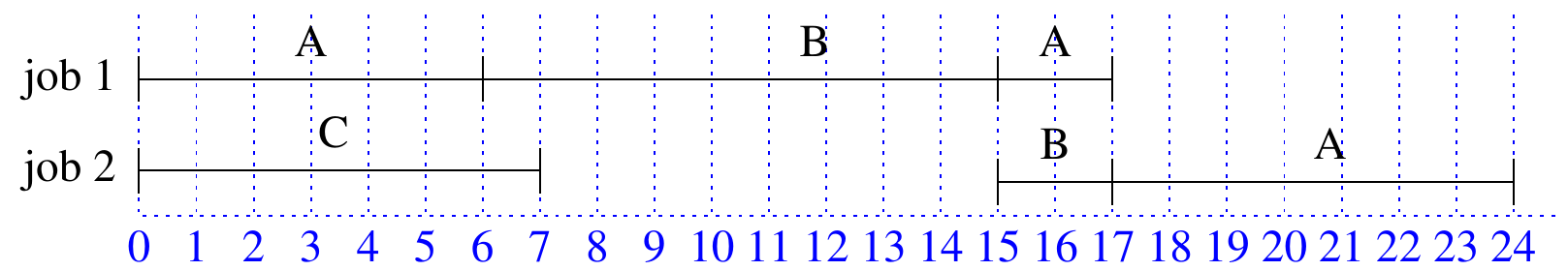
takes 24 time units and is not optimal.

We can formulate the problem in $ \IDL $. Given a set $ \JSJobs $ of jobs, we build a conjunction $ \JSForm $ as follows. First, we introduce a start time variable $ \JSStart{j}{t} $ for each task. The formula $ \JSForm $ then consists of the following conjuncts:

$ \JSStart{j}{t} \ge 0 $ for each task $ \JSTask{j}{t} $
$ \JSStart{j}{t} + \JSDur{j}{t} \le \JSStart{j}{t+1} $ for each task with $ t < \JSNofTasks{j} $ forces tasks in a job to be executed one after another
$ (\JSStart{j}{t} + \JSDur{j}{t} \le \JSStart{j’}{t’}) \lor (\JSStart{j’}{t’} + \JSDur{j’}{t’} \le \JSStart{j}{t}) $ for each pair $ \JSTask{j}{t} $, $ \JSTask{j’}{t’} $ of tasks with $ j \neq j’ $ and $ \JSMach{j}{t} = \JSMach{j’}{t’} $. Two tasks on different jobs using the same machine cannot be executed at the same time
$ \JSStart{j}{\JSNofTasks{j}} + \JSDur{j}{\JSNofTasks{j}} \le \JSBudget $ for each job $ j $, where $ \JSBudget $ is a variable.

The formula $ \JSForm \land {\JSBudget \Eq c} $ is $ \IDL $-satisfiable if and only if there is a schedule with total duration of $ c $ or less time units.

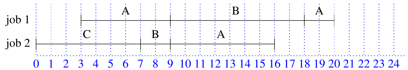
Consider again our concrete example set $ \JSJobs $ of two jobs, $ \JSJob{1} = \List{\Tuple{\textrm{A},6},\Tuple{\textrm{B},9},\Tuple{\textrm{A},2}} $ and $ \JSJob{2} = \List{\Tuple{\textrm{C},7},\Tuple{\textrm{B},2},\Tuple{\textrm{A},7}} $. For this we obtain the formula \begin{eqnarray*} \JSForm &=& {\JSStart{1}{1} \ge 0} \land {\JSStart{2}{1} \ge 0} \land {} \\ && {\JSStart{1}{1} + 6 \le \JSStart{1}{2}} \land {\JSStart{1}{2} + 9 \le \JSStart{1}{3}} \land {} \\ && {\JSStart{2}{1} + 7 \le \JSStart{2}{2}} \land {\JSStart{2}{2} + 2 \le \JSStart{2}{3}} \land {} \\ && {({\JSStart{1}{1} + 6 \le \JSStart{2}{3}} \lor {\JSStart{2}{3} + 7 \le \JSStart{1}{1}})} \land {} \\ && {({\JSStart{1}{2} + 9 \le \JSStart{2}{2}} \lor {\JSStart{2}{2} + 2 \le \JSStart{1}{2}})} \land {} \\ && {({\JSStart{1}{3} + 2 \le \JSStart{2}{3}} \lor {\JSStart{2}{3} + 7 \le \JSStart{1}{3}})} \land {} \\ && {\JSStart{1}{3} + 2 \le \JSBudget} \land {\JSStart{2}{3} + 7 \le \JSBudget} \end{eqnarray*} The smallest value $ c $ for which the formula $$\JSForm \land {\JSBudget \Eq c}$$ is $ \IDL $-satisfiable is $ 20 $.

Bit-Vectors¶

In some contexts, it is important to be able to perform bit-precise reasoning of hardware and software systems. The theory of bit-vectors allows this as in it the domains correspond to bounded, unsigned binary numbers with bit-level operations. Formally, a bit-vector of length $ n $ is a string $ x_{n-1}x_{n-2}…x_0 $ over the binary alphabet $ \Set{0,1} $. A bit-vector $ x_{n-1}x_{n-2}…x_0 $ represents the integer $ x_{n-1} 2^{n-1} + x_{n-2} 2^{n-2} + … + x_0 2^{0} $. For instance, $ 1001 $ represents the integer $ 1\times 8 + 0 \times 4 + 0 \times 2 + 1\times 1 = 9 $.

In the theory of bit-vectors $ \BVT $, the signature $ \BVSig $ includes, for each width $ n \ge 1 $,

the sort $ \BVS{n} $ for bit-vectors of width $ n $,
the predicate and function symbols for the usual bit-vector operations such as
- constants for bit-vector values,
- $ \BVLE{n} : \BVS{n} \times \BVS{n} $ for less-or-equal comparison,
- $ \BVAdd{n} : \BVS{n} \times \BVS{n} \to \BVS{n} $ for addition (modulo $ 2^n $), and
- $ \BVSL{n} : \BVS{n} \times \BVS{n} \to \BVS{n} $ for shifting left (pad with zeros).

The theory consists of the single intended interpretation in which the domain of $ \BVS{n} $ is the set of all bit-vectors of length $ n $, i.e., $ \Set{0,1}^n $, and the predicate and function symbols interpreted as expected, e.g., \begin{eqnarray*} 1100 \BVLE4 1001 &=& \False\\ 1100 \BVAdd4 1001 &=& 0101\\ 10110001 \BVSL8 00000010 &=& 11000100 \end{eqnarray*} When $ n $ is clear, the $ \BVS{n} $-subscripts can be omitted.

Example

The formula $$(x \ge y) \land (x + 3 \le y)$$ is $ \TLIA $-unsatisfiable but $$(x \BVGE{8} y) \land (x \BVAdd{8} 00000011 \BVLE{8} y)$$ is $ \BVT $-satisfiable due to possibility of overflows (e.g., $ x \mapsto 11111110 $ and $ y \mapsto 11110000 $).

Equality and Uninterpreted Functions¶

As its name implies, the theory of equality and uninterpreted functions and predicates allows the functions and predicates to be interpreted in all possible ways (except for the equality, which is always the element equality). Formally, assume a signature $ \Sig = \Tuple{\Set{\ElemSort},\Funcs,\Preds} $, where

$ \ElemSort $ is some sort,
$ \Funcs = \Set{f,g,h,f_1,…} $ is a countable set of function symbols, and
$ \Preds = \Set{\Eq,p,q,r,p_1,…} $ is a countable set of predicate symbols.

In our many-sorted FOL with the built-in equality symbol $ \Eq $, the $ \Sig $-theory $ \TEUF $ of uninterpreted functions (and predicates) consists of all possible $ \Sig $-structures. That is, the functions and predicate symbols are uninterpreted in the sense that any interpretation is suitable. The full $ \TEUF $-satisfiability is an undecidable problem but quantifier-free $ \TEUF $-satisfiability is decidable and allows efficient decision procedures (more about this in the next round).

Example

The quantifier-free formula $${g(x,y) \Eq g(f(x),y)} \land {f(x) \Neq x}$$ is $ \TEUF $-satisfiable. For instance, the interpretation $ \Interp $ with the domain $ \InterpDom = \Set{a,b} $, the function symbol interpretations $$\begin{array}{cc|cc}t_1&t_2&\InterpOf{f}(t_1)&\InterpOf{g}(t_1,t_2)\\ \hline a&a&b&a\\ a&b& &a\\ b&a&b&a\\ b&b& &a\\ \end{array}$$ and $ \Set{x \mapsto a, y \mapsto b} $ evaluates the formula to true as $ \InterpOf{g}(x,y) = \InterpOf{g}(\InterpOf{x},\InterpOf{y}) = \InterpOf{g}(a,b) = a = \InterpOf{g}(f(x),y) $, $ \InterpOf{f}(x) = b \neq \InterpOf{x} = a $.

Example

The formula \[{f(f(f(x))) \Eq x} \land {f(f(f(f(f(x))))) \Eq x} \land {f(x) \Neq x}\] is $ \TEUF $-unsatisfiable because

$ f(f(f(x))) \Eq x $ and $ f(f(f(f(f(x))))) \Eq x $ imply $ f(f(x)) \Eq x $, and
$ f(f(x)) \Eq x $ and $ f(f(f(x))) \Eq x $ imply $ f(x) \Eq x $.

Example

The formula $$\phi \quad = \quad {x \Eq y} \land {y \Eq z} \Implies g(f(x),y) \Eq g(f(z),x)$$ is $ \TEUF $-valid. We can prove this by assuming that there is an $ \TEUF $-interpretation $ \Interp $ such that $ \Interp \NotModels \phi $ and then showing that a contradiction follows.

If $ \Interp \NotModels \phi $, then $ \Interp \Models {x \Eq y} $ and $ \Interp \Models {y \Eq z} $.
Thus $ \InterpOf{x} = \InterpOf{y} = \InterpOf{z} $, implying $ \InterpOf{f}(\InterpOf{x}) = \InterpOf{f}(\InterpOf{z}) $ and $ \InterpOf{g}(\InterpOf{f}(\InterpOf{x}),\InterpOf{y}) = \InterpOf{g}(\InterpOf{f}(\InterpOf{z}),\InterpOf{x}) $
Therefore, $ \Interp \Models g(f(x),y) \Eq g(f(z),x) $ and $ \Interp \Models \phi $, a contradiction.

Note

In unsorted first-order logic without the built-in equality symbol, $ \EUF $ could be defined axiomatically with

the signature including the binary predicate $ \Eq $ and all predicate and function symbols, and
the following axioms:
- reflexivity: $ \forall x: x \Eq x $
- symmetry: $ \forall x,y: {x \Eq y} \Implies {y \Eq x} $
- transitivity: $ \forall x,y,z: {x \Eq y} \land {y \Eq z} \Implies {x \Eq z} $
- function congruence: $ \forall x_1,…,x_n,y_1,…,y_n: (\bigwedge_{i=1}^n x_i \Eq y_i) \Implies {f(x_1,…,x_n) \Eq f(y_1,…,y_n)} $ for each function symbol $ f $ with arity $ n $
- predicate congruence: $ \forall x_1,…,x_n,y_1,…,y_n: (\bigwedge_{i=1}^n x_i \Eq y_i) \Implies {(P(x_1,…,x_n) \Iff P(y_1,…,y_n))} $ for each predicate symbol $ P $ with arity $ n $

In this setting, one can only consider normal models where no distinct elements $ a $ and $ b $ satisfy $ a \Eq b $.

Example: Equivalence of simple programs¶

The following example is from D. Kroening and O. Strichman: Decision Procedures — An Algorithmic Point of View, Springer, 2008. Note that it can be seen as a simplified illustrative version of an approach for verifying microprocessor pipeline control, see:

J. R. Burch and D. L. Dill: Automatic verification of pipelined microprocessor control, Proc. CAV 1994, pages 68–80
R. E. Bryant et al: Modeling and Verifying Systems Using a Logic of Counter Arithmetic with Lambda Expressions and Uninterpreted Functions, Proc. CAV 2002, pages 78–92
H. Ganzinger et al: DPLL(T): Fast Decision Procedures, Proc. CAV 2004, pages 175–188.

Consider the following functions in C:

int power3(int in) {
  int out = in;
  for(int i = 0; i < 2; i++)
    out = out * in;
  return out;
}

and

int power3_new(int in) {
  int out = (in*in)*in;
  return out;
}

They should compute the same value (even if we replace * with any other binary function). We can verify their equivalence with $ \EUF $ as follows.

First, transform the programs into static single assignment (SSA) form, in which each variable is assigned only once, by (i) introducing new variables for intermediate results, and (ii) unwinding loops. Applying this to

int power3(int in) {
  int out = in;
  for(int i = 0; i < 2; i++)
    out = out * in;
  return out;
}

gives

int power3(int in) {
  int out1 = in;
  int out2 = out1 * in;
  int out3 = out2 * in;
  return out3;
}

while the other program

int power3_new(int in) {
  int out = (in*in)*in;
  return out;
}

is already in the SSA form.

Next, we interpret the assignments as equations. The first program

int power3(int in) {
  int out1 = in;
  int out2 = out1 * in;
  int out3 = out2 * in;
  return out3;
}

corresponds to the equations \begin{eqnarray*} \Out_1 &\Eq& \In \\ \Out_2 &\Eq& \Out_1 * \In \\ \Out_3 &\Eq& \Out_2 * \In \end{eqnarray*} while the second program

int power3_new(int in) {
  int out = (in*in)*in;
  return out;
}

is captured by a single equation \begin{eqnarray*} \Out’ &\Eq& (\In * \In) * \In \end{eqnarray*}

Under the semantics of the C language types and operands (the theory of bit-vectors introduced later in this round), the formula \begin{eqnarray*} &&{\Out_1 \Eq \In} \land {\Out_2 \Eq \Out_1 * \In} \land {\Out_3 \Eq \Out_2 * \In} \land {}\\ &&{\Out’ \Eq (\In * \In) * \In}\\ &\Implies& {\Out_3 \Eq \Out’} \end{eqnarray*} is valid if and only if the C functions are equivalent.

However, in this simple example, the full semantics of C operands is not needed. Because $ \TEUF $-interpretations “include” the precise bit-vector ones, we can try replacing the interpreted functions with uninterpreted ones. Thus in this example the function $ * $ is replaced with an uniterpreted binary function $ f $ and

$ {\Out_1 \Eq \In} \land {\Out_2 \Eq \Out_1 * \In} \land {\Out_3 \Eq \Out_2 * \In} $ becomes $ {\Out_1 \Eq \In} \land {\Out_2 \Eq f(\Out_1,\In)} \land {\Out_3 \Eq f(\Out_2,\In)} $, and
$ \Out’ \Eq (\In * \In) * \In $ becomes $ \Out’ \Eq f(f(\In,\In),\In) $.

Now if the formula \begin{eqnarray*} &&{\Out_1 \Eq \In} \land {\Out_2 \Eq f(\Out_1,\In)} \land {\Out_3 \Eq f(\Out_2,\In)} \land {}\\ &&{\Out’ \Eq f(f(\In,\In),\In)}\\ &\Implies& {\Out_3 \Eq \Out’} \end{eqnarray*} is $ \TEUF $-valid, then the C functions are equivalent. But observe that if the $ \TEUF $-formula is not valid, we cannot say anything about the validity of bit-vector formula.

To check the validity of a formula with an SMT solver, we can negate the formula and check whether it is unsatisfiable. Therefore, if the negated formula \begin{eqnarray*} &&{\Out_1 \Eq \In} \land {\Out_2 \Eq f(\Out_1,\In)} \land {\Out_3 \Eq f(\Out_2,\In)} \land {}\\ &&{\Out’ \Eq f(f(\In,\In),\In)}\\ &\land& {\Out_3 \Neq \Out’} \end{eqnarray*} is $ \TEUF $-unsatisfiable, then the C functions are equivalent.

Arrays¶

In applications areas such as program verification, one may need to model memory accesses or use of dictionaries and arrays. They can captured with a functional-style abstract data type for arrays having the following interface:

$ \Read{a}{i} $ gives the element at index $ i $ of the array $ a $, and
$ \Write{a}{i}{v} $ gives an array similar to the array $ a $ except that the index $ i $ contains the element $ v $.

Formally, the signature $ \ArrSig $ has the sorts

$ \IndexSort $ for indices,
$ \ElemSort $ for elements stored in the array, and
$ \ArraySort $ for $ \IndexSort $-indexed arrays of $ \ElemSort $-elements,

and the function symbols

$ \ReadF : \ArraySort \times \IndexSort \to \ElemSort $, and
$ \WriteF: \ArraySort \times \IndexSort \times \ElemSort \to \ArraySort $.

The (non-extensional) theory $ \TArrays $ of arrays is usually defined axiomatically, the axioms being:

read over write 1: $ \A{a}{\ArraySort}{\A{i,j}{\IndexSort}{\A{v}{\ElemSort}{{i \Eq j} \Implies {\Read{\Write{a}{i}{v}}{j} \Eq v}}}} $
read over write 2: $ \A{a}{\ArraySort}{\A{i,j}{\IndexSort}{\A{v}{\ElemSort}{{i \Neq j} \Implies \Read{\Write{a}{i}{v}}{j} \Eq \Read{a}{j}}}} $

The first one states that if we write an element $ v $ to an index $ i $ of an array $ a $, then reading the same index in the resulting array will give $ v $. The second one states that if we write an element $ v $ to an index $ i $ of an array $ a $, then reading some other index in the resulting array will give the element that $ a $ had before the write operation.

When showing the satisfiability of a formula, it is enough to give one interpretation extending some structure in the theory.

Example

Consider the formula \begin{eqnarray*} (c \Implies {b \Eq \Write{a}{i}{v}}) \land ({\neg c} \Implies {b \Eq \Write{a}{i}{w}}) &\Implies&\\\\ ({\Read{b}{i} \Eq v} \lor {\Read{b}{i} \Eq w}). \end{eqnarray*} It is $ \TArrays $-satisfiable because we can choose the following structure $ \Interp $:

The domain of the index sort $ \IndexSort $ is $ \DomOf{\IndexSort} = \Set{\DA,\DB,\DC,\DD} $. These symbols were selected only to show that the index set does not have to be integers.
The domain of the element sort $ \ElemSort $ is $ \DomOf{\ElemSort} = \Set{0,1,2,3,4,5} $.
The domain of the array sort $ \DomOf{\ArraySort} $ consists of all the functions from $ \DomOf{\IndexSort} $ to $ \DomOf{\ElemSort} $.
$ \InterpOf{\ReadF}(a,i) = a(i) $, and
$ \InterpOf{\WriteF}(a,i,v) $ is the function $ b = \Substf{a}{i}{v} $ for which $ b(i) = v $ and $ b(j) = a(j) $ for all $ j \neq i $.

For this structure it is easy to see that the axioms hold and thus the structure belongs to the theory $ \TArrays $.

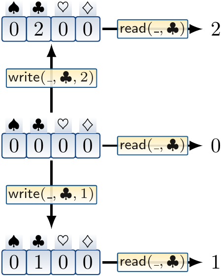
Now the interpretation that extends $ \Interp $ by $ c \mapsto \True $, $ i \mapsto \DB $, $ v \mapsto 1 $, $ w \mapsto 2 $, $ a \mapsto \Set{\DA\mapsto 0, \DB\mapsto 0, \DC\mapsto 0, \DD\mapsto 0} $, and $ b \mapsto \Set{\DA\mapsto 0, \DB\mapsto 1, \DC\mapsto 0, \DD\mapsto 0} $ clearly evaluates the formula to true.

When showing unsatisfiability (or validity) of formulas modulo an axiomatically defined theory, one must show that the formula is unsatisfiable (or valid) in all structures allowed by the axioms.

Example

The formula \begin{eqnarray*} (c \Implies {b \Eq \Write{a}{i}{v}}) \land ({\neg c} \Implies {b \Eq \Write{a}{i}{w}}) &\Implies&\\\\ ({\Read{b}{i} \Eq v} \lor {\Read{b}{i} \Eq w}) \end{eqnarray*} is $ \TArrays $-valid because if \[\Interp \Models (c \Implies b\Eq\WriteF(a,i,v)) \land ({\neg c} \Implies b\Eq\WriteF(a,i,w))\] for some $ \TArrays $-interpretation $ \Interp $, then either $ \InterpOf{b} = \InterpOf{\WriteF}(\InterpOf{a},\InterpOf{i},\InterpOf{v}) $ or $ \InterpOf{b} = \InterpOf{\WriteF}(\InterpOf{a},\InterpOf{i},\InterpOf{w}) $. Due to the “Read over write 1” axiom, $ \InterpOf{\ReadF}(\InterpOf{\WriteF}(\InterpOf{a},\InterpOf{i},\InterpOf{v}),\InterpOf{i}) = \InterpOf{v} $ and $ \InterpOf{\ReadF}(\InterpOf{\WriteF}(\InterpOf{a},\InterpOf{i},\InterpOf{w}),\InterpOf{i}) = \InterpOf{w} $. Thus $ \InterpOf{\ReadF}(\InterpOf{b},\InterpOf{i}) = \InterpOf{v} $ or $ \InterpOf{\ReadF}(\InterpOf{b},\InterpOf{i}) = \InterpOf{w} $ (or both), and $$\Interp \Models (\Read{b}{i}\Eq v \lor \Read{b}{i}\Eq w)$$ holds as well.

There is a small catch in the axiomatic definition given above. namely, the resulting theory $ \TArrays $ does not state when two arrays have the same content (i.e., are equal).

Example

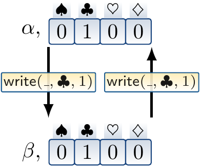
Consider the formula \[{\Read{a}{i} \Eq v} \Implies {\Write{a}{i}{v} \Eq a}\] stating that “if an array $ a $ already contains an element $ v $ at the index $ i $, then writing the same element in that index again should give the same array”. It is not $ \TArrays $-valid because the axioms allow structures with multiple copies of the same array. For instance, we may choose the following structure $ \Interp $ having “$ \alpha $ and $ \beta $ copies” of arrays:

The domain of the index sort $ \IndexSort $ is $ \DomOf{\IndexSort} = \Set{\DA,\DB,\DC,\DD} $
The domain of the element sort $ \ElemSort $ is $ \DomOf{\ElemSort} = \Set{0,1,2,3,4,5} $.
The domain of the array sort $ \DomOf{\ArraySort} $ is $ \Setdef{\Tuple{\alpha,f},\Tuple{\beta,f}}{f \in \Functions{\DomOf{\IndexSort}}{\DomOf{\ElemSort}}} $.
$ \InterpOf{\ReadF}(\Tuple{\alpha,a},i) = a(i) $,
$ \InterpOf{\ReadF}(\Tuple{\beta,a},i) = a(i) $,
$ \InterpOf{\WriteF}(\Tuple{\alpha,a},i,v) = \Tuple{\beta, \Substf{a}{i}{v}} $, and
$ \InterpOf{\WriteF}(\Tuple{\beta,a},i,v) = \Tuple{\alpha, \Substf{a}{i}{v}} $.

For this structure it is easy to see that the axioms hold and thus the structure belongs to the theory $ \TArrays $.

Now the interpretation that extends $ \Interp $ by $ i \mapsto \DB $, $ v \mapsto 1 $, $ a \mapsto \Tuple{\alpha,\Set{\DA\mapsto 0, \DB\mapsto 1, \DC\mapsto 0, \DD\mapsto 0}} $ clearly evaluates the formula to false as $ \Write{a}{i}{v} = \Tuple{\beta, \Set{\DA\mapsto 0, \DB\mapsto 1, \DC\mapsto 0, \DD\mapsto 0}} $.

To capture array equality, we can add another axiom

extensionality: $ \A{a,b}{\ArraySort}{\left(\A{i}{\IndexSort}{\Read{a}{i} \Eq \Read{b}{i}}\right) \Implies {a \Eq b}} $

to $ \TArrays $ to obtain the extensional theory of arrays $ \TArraysExt $. This axiom rules out such “spurious copies” of arrays.