Theory Combination
So far we have considered only the case in which all the terms in the formulas are from a single theory. However, sometimes we would like to use several theories in a formula and write something like $${1 \le x} \land {x \le 2} \land {w_1 \Eq 1} \land {w_2 \Eq 2} \land {f(x) \Neq f(w_1)} \land {f(x) \Neq f(w_2)}$$ In the following introductory text, we consider satisfiability of quantifier-free conjunctions of literals; the approach generalizes to full Boolean case by using the CDCL(\( \Th \)) approach or DNF translation.
Sometimes combining theories is an easy task. Two theories, \( \ThI1 \) and \( \ThI2 \), are strongly disjoint if they do not share any sorts, and consequently no variables or function or predicate symbols. For such theories, one cannot mix different theories inside an atom. Thus the atoms can be fully separated into disjoint theory parts and the parts can be handled separately.
Example
In the formula $${x + 2y \le z} \land {y-z \Eq 0} \land {\Car(l) \Eq e} \land {\Cdr(l) \Eq l}$$ the linear arithmetic \( \TLIA \) part and the list \( \ThCons \) part (recall the exercise in Round 8) are fully separate if the element and list sorts in \( \ThCons \) are not \( \IntsSort \). Therefore, the formula is \( (\TLIA \TComb \ThCons) \)-satisfiable if and only if
\( {x + 2y \le z} \land {y - z \Eq 0} \) is \( \TLIA \)-satisfiable and
\( {\Car(l) \Eq e} \land {\Cdr(l) \Eq l} \) is \( \ThCons \)-satisfiable.
However, in general theory combination is a more complex topic.
The Nelson–Oppen Theory Combination Method
In many cases, the combined theories are not strongly disjoint but still have some properties that can be exploited when building solvers for the combined theory. Below we present the currently mostly used theory combination method that works for several theory combinations. To do that, we first need two additional definitions of “signature disjointness” and “stably infiniteness”.
Definition
Two theories, \( \ThI1 \) and \( \ThI2 \), are signature disjoint if they do not share any function or predicate symbols except for the equality symbol.
Example
Consider the theory \( \TLIA \) of linear arithmetic over integers and the theory \( \TEUF \) of uninterpreted functions with its element sort \( \ElemSort \) equal to \( \IntsSort \). One can now write formulas such as $${f(x+1) \le 3} \land {3f(y) \Eq 7}$$ The theories are signature disjoint as, intuitively,
\( \TEUF \) does not place any restrictions on the element sort, and
\( \TLIA \) does not consider the uninterpreted function and predicate symbols.
Formally, the axiomatic definition of \( \TEUF \) does not refer to the constants (\( 0 \) and \( 1 \)), functions (such as \( + \)), or predicates (\( < \)) other than the equality used in the axiomatic definition of \( \TLIA \). Vice versa, the axiomatic definition of \( \TLIA \) does not use the function symbols (such as \( f \)) or predicates appearing in the axiomatic definition of \( \TEUF \).
As shown in the next example, the straightforward combination of decision procedures does not work when variables or symbols are shared.
Example
Consider the conjunctive \( (\TEUF \TComb \TLIA) \)-formula $${1 \le x} \land {x \le 2} \land {w_1 \Eq 1} \land {w_2 \Eq 2} \land {f(x) \Neq f(w_1)} \land {f(x) \Neq f(w_2)}$$ where \( f: \IntsSort \to \IntsSort \). Now
The “\( \TEUF \)-part” \( {f(x) \Neq f(w_1)} \land {f(x) \Neq f(w_2)} \) is satisfiable as \( \InterpI{1} = \{x \mapsto 3, w_1 \mapsto 1, w_2 \mapsto 2, f \mapsto \{1 \mapsto 4, 2 \mapsto 2, 3 \mapsto 6,…\}\} \) evaluates it to true.
The “\( \TLIA \)-part” \( {1 \le x} \land {x \le 2} \land {w_1 \Eq 1} \land {w_2 \Eq 2} \) is satisfiable because \( \InterpI2 = \{x \mapsto 1, w_1 \mapsto 1, w_2 \mapsto 2\} \) evaluates it to true.
But these two interpretations are not compatible as they give different values to the variable \( x \).
In fact, the combination of the \( \TEUF \)- and \( \TLIA \)-parts, i.e. the whole formula, is unsatisfiable.
Definition: Stably Infiniteness
A theory \( \Th \) with signature \( \Sig \) is stably infinite if for every \( \Th \)-satisfiable \( \Sigma \)-formula \( \phi \) there is a \( \Th \)-model in which all the domains are infinite.
As an example, the theory of bit-vectors is not stably infinite while the theories \( \TEUF \), \( \TLIA \), \( \TLRA \) and so on are stably infinite. Intuitively, the stable infiniteness quarantees that combination method below always has enough “extra values” available.
The Abstract Method
As mentioned above, the Nelson–Oppen method is the current main method for combining theories. Its main idea is that for theories with some properties, it is enough to ensure that the different theory parts agree on the equalities between shared variables. In the following, we will gradully present an abstract version of the method for two theories, \( \ThI1 \) and \( \ThI2 \) with signatures \( \SigI1 \) and \( \SigI2 \), respectively, but the idea generalizes to multiple theories as well.
The goal of the method is to decide the \( (\ThI1 \TComb \ThI2) \)-satisfiability of a conjunction \( \phi \). The requirements are:
\( \ThI1 \) and \( \ThI2 \) are signature disjoint
\( \ThI1 \) and \( \ThI2 \) are stably infinite
The conjunction \( \phi \) should be in form \( \phi_1 \land \phi_2 \), where
\( \phi_1 \) is a \( \SigI1 \)-conjunction, and
\( \phi_2 \) is a \( \SigI2 \)-conjunction
This can be achieved with purification, explained next.
Purification
Given a \( (\SigI1 \cup \SigI2) \)-conjunction \( \phi \), purification transforms \( \phi \) into a \( \SigI1 \)-conjunction \( \phi_1 \) and a \( \SigI2 \)-conjunction \( \phi_2 \) such that \( \phi \) is \( (\ThI1 \cup \ThI2) \)-satisfiable if and only if \( \phi_1 \land \phi_2 \) is \( (\ThI1 \cup \ThI2) \)-satisfiable. That is, the conjunction will be divided in two parts that only concern a single theory but may share some variables. The diea of the purification process is simple: if an atom contains function or predicate symbols from two theories, substitute the other term with a new variable that is defined, in a separate atom, to be equal to that term. More precisely, the procedure can be described as follows. Let \( i,j \in \Set{1,2} \) with \( i \neq j \). Repeat the following as long as possible
If \( f \in \SigI{i} \) and \( g \in \SigI{j} \) and \( f(…,g(…),…) \) is a term in \( \phi \), rewrite the term into \( f(…,t,…) \) and conjunct \( \phi \) with \( (t \Eq g(…)) \).
If \( f \in \SigI{i} \) and \( g \in \SigI{j} \) and \( f(….) \Eq g(…) \) is a term in \( \phi \), rewrite the term into \( t \Eq g(…) \) and conjunct \( \phi \) with \( (t \Eq f(…)) \).
If \( p \in \SigI{i} \), \( p \neq {\Eq} \) and \( f \in \SigI{j} \) and \( p(…,f(…),…) \) is an atom in \( \phi \), rewrite the atom into \( p(…,t,…) \) and conjunct \( \phi \) with \( (t \Eq f(…)) \).
In every step above, \( t \) is a new fresh variable not yet occurring in \( \phi \). Finally, \( \phi_1 \) is the conjunction of all the atoms in the resulting \( \phi \) that do not contain \( \SigI2 \)-symbols (and vice versa for \( \phi_2 \)).
Example
Consider the \( (\TLIA \TComb \TEUF) \)-conjunction $$\phi \quad\Def\quad {f(x+1) \le 3} \land {3f(y) \Eq 7}$$ Applying purification to it may produce $${t_2 \le 3} \land {3t_3 \Eq 7} \land {t_1 \Eq x+1} \land {t_2 \Eq f(t_1)} \land {t_3 \Eq f(y)}$$ and the theory parts are thus \begin{eqnarray*} \phi_\LIA &\Def& {t_2 \le 3} \land {3t_3 \Eq 7} \land {t_1 \Eq x+1}\\\\ \phi_\EUF &\Def& {t_2 \Eq f(t_1)} \land {t_3 \Eq f(y)} \end{eqnarray*}
In fact, purification can be applied to a non-conjunctive formulas as well, resulting in a formula where each atom contains symbols (other than \( \Eq \)) from a single theory only. Therefore, in the DPLL(\( \Th \)) framework one can apply the purification once in the beginning at the formula level. Furthermore, the size of the purified formula is linear in the size of the original formula.
Example
Consider the \( (\TLIA \TComb \TEUF) \)-formula $${f(x+1) \le 3} \Implies {3f(y) \Eq 7}$$ Applying purification to it may produce $$({t_2 \le 3} \Implies {3t_3 \Eq 7}) \land {t_1 \Eq x+1} \land {t_2 \Eq f(t_1)} \land {t_3 \Eq f(y)}$$
Implementing the Abstract Method
Implementing the abstract method simply going through all the possible partitions is not practical at all. This is because the number of possible partitions of a set with \( n \) elements is known as the Bell number \( B_n \) and such numbers grow very fast, e.g., \( B_{20} = 51,724,158,235,372 \). So how can the abstract method be realized efficiently? There are basically two ways when we consider the CDCL(\( \Th \)) framework with a propositional SAT solver and theory solvers for the theories \( \ThI1 \) and \( \ThI2 \).
The Equality Detection and Propagation Method
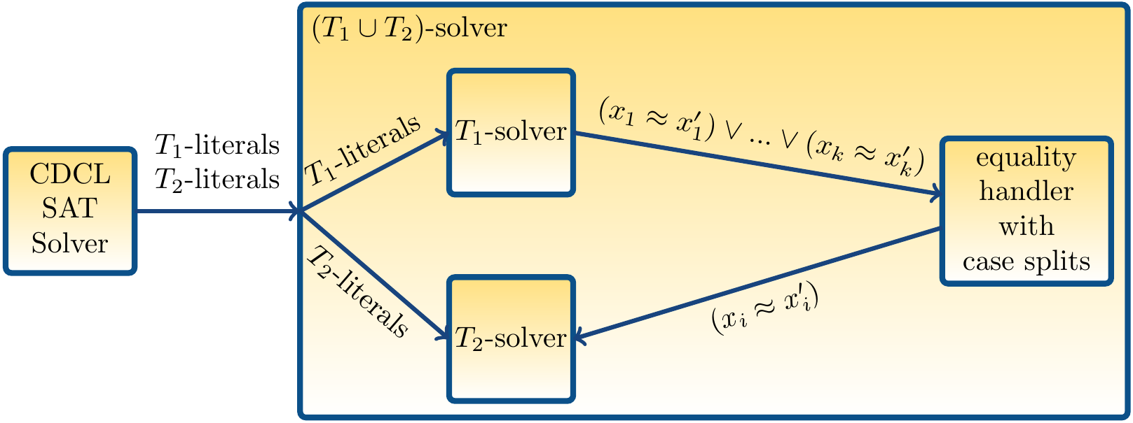
In the first approach for implementing the abstract Nelson–Oppen method, one combines the solvers for the theories \( \ThI1 \) and \( \ThI2 \) into a new one for \( \ThI1 \cup \ThI2 \). The component theory solvers for \( \ThI{i} \), \( i \in \Set{1,2} \), shall implement detection of disjunctions of equalities: given a conjunction \( \phi_i \) of atoms, detect the (minimal) disjunctions \( (x_1 \Eq x’_1) \lor … \lor (x_k \Eq x’_k) \) such that
\( x_1,…,x_k,x’_1,…,x’_k \) are shared variables, and
\( \phi_i \ThIModels{i} (x_1 \Eq x’_1) \lor … \lor (x_k \Eq x’_k) \)
The detected disjunctions of equalities between shared variables are propagated to other theory solver. If the disjunction has more than one disjunct, case splitting must be done, i.e., the new combined theory solver tries to find a model by considering each disjunct \( x_j \Eq x’_j \) in turn. A high-level schematic picture of this approach is shown below.
Example
Consider the \( (\TEUF \TComb \TLIA) \)-conjunction \( \NOF \Def \NOFEUF \land \NOFLIA \) with
\( \NOFEUF \Def {{f(x) \Neq f(w_1)} \land {f(x) \Neq f(w_2)}} \), and
\( \NOFLIA \Def {1 \le x} \land {x \le 2} \land {w_1 \Eq 1} \land {w_2 \Eq 2} \).
In the combined theory solver,
the literals in \( \NOFEUF \) are asserted in the \( \TEUF \)-solver: \( \TEUF \)-satisfiability but no implied equalities is reported
the literals in \( \NOFLIA \) are asserted in the \( \TLIA \)-solver: \( \TLIA \)-satisfiability and the implied disjunction \( (x \Eq w_1) \lor (x \Eq w_2) \) over the shared variables is reported
the combined theory solver performs case split:
the equality \( (x \Eq w_1) \) is asserted in the \( \TEUF \)-solver: \( \TEUF \)-unsatisfiability is reported as \( {f(x) \Neq f(w_1)} \land {x \Eq w_1} \) is \( \TEUF \)-unsatisfiable
the equality \( (x \Eq w_2) \) is asserted in the \( \TEUF \)-solver: \( \TEUF \)-unsatisfiability is reported as \( {f(x) \Neq f(w_2)} \land {x \Eq w_2} \) is \( \TEUF \)-unsatisfiable
The combined solver deduces that \( \NOF \) is unsatisfiable
The drawback of this method is that one must augment the theory solvers with the capability of detecting (preferably minimal) implied disjunctions of equalities.
The Delayed Theory Combination Method
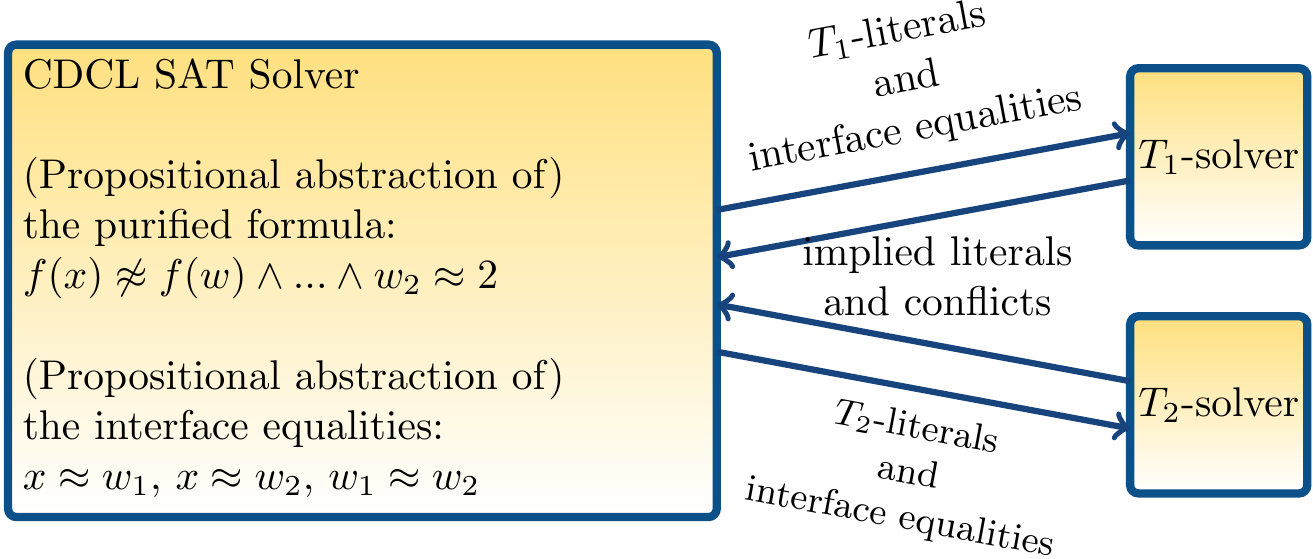
As mentioned above, building decision procedures that can detect (disjunctions of) equalities can be more challenging than the ones without this capability. In the “delayed theory combination” method, the idea is to use regular theory solvers and let the CDCL SAT solver take care of the equality literal handling as follows.
Consider the CDCL(\( \Th \)) approach but now with two theory solvers, one for \( \ThI1 \) and one for \( \ThI2 \).
In the beginning, introduce the \( \frac{n(n-1)}{2} \) possible interface equality atoms of the form \( x \Eq y \) over the \( n \) shared variables
Let the SAT solver decide values for them (i.e., to guess an arrangement) and then pass them to the theory solvers as usual. In this way, the theory solvers don’t have to implement equality propagation because they receive the equalities from the SAT solver. Furthermore, the SAT solver can learn infeasible equality combinations because it receives conflicts involving the interface equalities from the theory solvers.
A high-level schematic picture of this approach is shown below.
Example
Consider again the \( (\TEUF \TComb \TLIA) \)-conjunction \( \NOF \Def \NOFEUF \land \NOFLIA \) with
\( \NOFEUF \Def {{f(x) \Neq f(w_1)} \land {f(x) \Neq f(w_2)}} \), and
\( \NOFLIA \Def {1 \le x} \land {x \le 2} \land {w_1 \Eq 1} \land {w_2 \Eq 2} \).
In the beginning, the SAT solver introduces the 3 interface equalities $$x \Eq w_1, x \Eq w_2, w_1 \Eq w_2$$ Here is a possible run of the method:
All the literals in the conjunction are asserted to true in the SAT solver.
The literals in \( \NOFEUF \) are asserted in the \( \TEUF \)-solver: \( \TEUF \)-satisfiability is reported.
The literals in \( \NOFLIA \) are asserted in the \( \TLIA \)-solver: \( \TLIA \)-satisfiability is reported.
The SAT solver guesses that \( x \Eq w_1 \) is true.
The literal \( x \Eq w_1 \) is asserted in the \( \TEUF \)-solver: \( \TEUF \)-unsatisfiability with the theory conflict \( {f(x) \Neq f(w_1)} \land {x \Eq w_1} \) is reported.
The SAT solver analyzes the conflict clause \( {f(x) \Eq f(w_1)} \lor {x \Neq w_1} \), backtracks and unit propagates \( (x \Neq w_1) \).
The literal \( x \Neq w_1 \) is asserted in the \( \TEUF \)-solver: \( \TEUF \)-satisfiability is reported.
The literal \( x \Neq w_1 \) is asserted in the \( \TLIA \)-solver: \( \TLIA \)-satisfiability is reported.
The SAT solver guesses that \( x \Eq w_2 \) is true.
The literal \( x \Eq w_2 \) is asserted in the \( \TEUF \)-solver: \( \TEUF \)-unsatisfiability with the theory conflict \( {f(x) \Neq f(w_2)} \land {x \Eq w_2} \) is reported.
The SAT solver analyzes the conflict clause \( {f(x) \Eq f(w_2)} \lor {x \Neq w_2} \), backtracks and unit propagates \( (x \Neq w_2) \).
The literal \( x \Neq w_2 \) is asserted in the \( \TEUF \)-solver: \( \TEUF \)-satisfiability is reported.
The literal \( x \Neq w_2 \) is asserted in the \( \TLIA \)-solver: \( \TLIA \)-unsatisfiability with the theory conflict \( {1 \le x} \land {x \le 2} \land {w_1 \Eq 1} \land {w_2 \Eq 2} \land {x \Neq w_1} \land {x \Neq w_2} \) is reported.
The SAT solver analyzes the conflict and reports unsatisfiability.
Some notes: convexity and complexity
Convex theories are a special subclass for which the Nelson–Oppen combination with equality detection and propagation can be made simpler.
Definition: Convexity
A theory \( \Th \) is convex if $$\phi \ThModels \bigvee_{i=1}^n(u_i \Eq v_i) \text{ implies } \phi \ThModels (u_j \Eq v_j)\text{ for some \( j \in \Set{1,…,n} \)}$$ holds for all conjunctive \( \Sig \)-formulas \( \phi \), for all variables \( u_i \) and \( v_i \), and for all positive \( n \)
If both combined theories are convex, the equality detection and propagation approach has to only detect and propagate implied equalities, not disjunctions of equalities. As an example, linear arithmetic over reals and \( \EUF \) are convex theories.
Example
Linear arithmetic over integers is not convex as, for instance, $${0 \le x} \land {x \le 1} \land {y \Eq 0} \land {z \Eq 1} \LIAModels {x \Eq y} \lor {x \Eq z}$$ but neither
\( {0 \le x} \land {x \le 1} \land {y \Eq 0} \land {z \Eq 1} \LIAModels {x \Eq y} \) nor
\( {0 \le x} \land {x \le 1} \land {y \Eq 0} \land {z \Eq 1} \LIAModels {x \Eq z} \) holds
Assume that \( \ThI1 \) and \( \ThI2 \) are signature disjoint, stably infinite theories.
Theorem
If \( \ThI1 \) and \( \ThI2 \) are convex and both have polynomial time decision procedures, then the equality-propagating Nelson-Oppen procedure is a polynomial time decision procedure for \( \ThI1 \cup \ThI2 \).
Theorem
If \( \ThI1 \) and \( \ThI2 \) are non-convex and both have nondeterministic polynomial time decision procedures, then the equality-propagating Nelson-Oppen procedure is a nondeterministic polynomial time decision procedure for \( \ThI1 \cup \ThI2 \).
Combining EUF with another theory
One interesting special case is the combination \( \EUF \TComb \Th \) of the theory \( \EUF \) of uninterpreted functions with some other theory \( \Th \). Of course, one can use the Nelson–Oppen method as described earlier. But one can also use Ackermann’s reduction to get rid of the uninterpreted function and predicate symbols. That is, the \( (\EUF \TComb \Th) \)-satisfiability problem can be reduced to the \( \Th \)-satisfiability problem.
Given a formula \( \phi \) involving uninterpreted function and/or predicate symbols, Ackermann’s reduction translates \( \phi \) into a formula \( \phi’ \) that
does not involve any uninterpreted function or predicate symbols, and
is satisfiable if and only if \( \phi \) is.
The constructed formula \( \phi’ \) is of form \( \Flat \land \Cong \), where
\( \Flat \Def \Ack{\phi} \) is a “flattened” version of \( \phi \), in which all the topmost uninterpreted function and predicate applications are replaced with new variables, and
\( \Cong \) is a conjunction of implications that force function and predicate congruence.
Formally, the translation \( \Ack{\phi} \) is defined as follows:
\( \Ack{p(t_1,…,t_n)} \) is a new Boolean variable \( \VVar{p(t_1,…,t_n)} \) for an uninterpreted \( n \)-ary predicate symbol \( p \),
\( \Ack{f(t_1,…,t_n)} \) is a new variable \( \VVar{f(t_1,…,t_n)} \) of sort \( \Sort \) for an uninterpreted \( n \)-ary, \( n \ge 1 \), function symbol \( f \) of type \( \SortI{1} \times … \times \Sort_n \to \Sort \),
\( \Ack{c} \Def c \) for each constant \( c \),
\( \Ack{x} \Def x \) for each variable \( x \), and
otherwise \( \Ack{\phi} \) is homomorphic wrt Boolean connectives, the equality symbol \( \Eq \), and interpreted functions \( f \) and \( p \), meaning that, e.g., \( \Ack{\phi_1 \land \phi_2} \Def \Ack{\phi_1} \land \Ack{\phi_2} \) and \( \Ack{t_1 + t_2} = {\Ack{t_1} + \Ack{t_2}} \).
The formula \( \Cong \) is a conjunction of implications that force function and predicate congruence:
for each pair, \( f(t_1,…,t_n) \) and \( f(t’_1,…,t’_n) \) with \( n \ge 1 \), of uninterpreted function applications in \( \phi \), \( \Cong \) contains the implication $$(\bigwedge_{i=1}^n {\Ack{t_1} \Eq \Ack{t’_1}}) \Implies {\VVar{f(t_1,…,t_n)} \Eq \VVar{f(t’_1,…,t’_n)}}$$
for each pair, \( p(t_1,…,t_n) \) and \( p(t’_1,…,t’_n) \), of uninterpreted predicate applications in \( \phi \), \( \Cong \) contains the implication $$(\bigwedge_{i=1}^n {\Ack{t_1} \Eq \Ack{t’_1}}) \Implies (\VVar{p(t_1,…,t_n)} \Iff \VVar{p(t’_1,…,t’_n)})$$
Example
Consider again the \( (\TLIA \TComb \TEUF) \)-formula $${f(x+1) \le 3} \Implies {3f(y) \Eq 7}$$ Applying Ackermann’s reduction to it produces $$({v_{f(x+1)} \le 3} \Implies {3v_{f(y)} \Eq 7}) \land ({x+1 \Eq y} \Implies {v_{f(x+1)} \Eq v_{f(y)}})$$ and thus the \( (\TLIA \TComb \TEUF) \)-satisfiability problem is reduced to a \( \TLIA \)-satisfiability problem
Example
If we apply the reduction to the formula \begin{eqnarray*} \phi &=&{\Out_1 \Eq \In} \land {\Out_2 \Eq f(\Out_1,\In)} \land {\Out_3 \Eq f(\Out_2,\In)} \land {}\\\\ &&{\Out’ \Eq f(f(\In,\In),\In)} \land {\Out_3 \Neq \Out’} \end{eqnarray*} discussed in Round 8, we get \begin{eqnarray} \Flat &\Def&{\Out_1 \Eq \In} \land {\Out_2 \Eq \VVar{f(\Out_1,\In)}} \land {\Out_3 \Eq \VVar{f(\Out_2,\In)}} \land {}\\\\ &&{\Out’ \Eq \VVar{f(f(\In,\In),\In)}} \land {\Out_3 \Neq \Out’}\\\\ \Cong &\Def& ({\Out_1 \Eq \Out_2} \land {\In \Eq \In} \Implies {\VVar{f(\Out_1,\In)} \Eq \VVar{f(\Out_2,\In)}}) \land {} \label{EX:fc1}\\\\ & & ({\Out_1 \Eq \In} \land {\In \Eq \In} \Implies {\VVar{f(\Out_1,\In)} \Eq \VVar{f(\In,\In)}}) \land {} \label{EX:fc2}\\\\ & & ({\Out_1 \Eq \VVar{f(\In,\In)}} \land {\In \Eq \In} \Implies {\VVar{f(\Out_1,\In)} \Eq \VVar{f(f(\In,\In),\In)}}) \land {}\\\\ & & ({\Out_2 \Eq \In} \land {\In \Eq \In} \Implies {\VVar{f(\Out_2,\In)} \Eq \VVar{f(\In,\In)}}) \land {}\\\\ & & ({\Out_2 \Eq \VVar{f(\In,\In)}} \land {\In \Eq \In} \Implies {\VVar{f(\Out_2,\In)} \Eq \VVar{f(f(\In,\In),\In)}}) \label{EX:fc5}\\\\ & & ({\In \Eq \VVar{f(\In,\In)}} \land {\In \Eq \In} \Implies {\VVar{f(\In,\In)} \Eq \VVar{f(f(\In,\In),\In)}}) \label{EX:fc6} \end{eqnarray} Now \( \Flat \land \Cong \) is unsatisfiable as
\( \Out_1 \Eq \In \) in \( \Flat \) and \( {\Out_1 \Eq \In} \land {\In \Eq \In} \Implies {\VVar{f(\Out_1,\In)} \Eq \VVar{f(\In,\In)}} \) in \( \Cong \) imply \( \VVar{f(\Out_1,\In)} \Eq \VVar{f(\In,\In)} \),
\( \VVar{f(\Out_1,\In)} \Eq \VVar{f(\In,\In)} \) and \( \Out_2 \Eq \VVar{f(\Out_1,\In)} \) in \( \Flat \) imply \( \Out_2 \Eq \VVar{f(\In,\In)} \),
\( \Out_2 \Eq \VVar{f(\In,\In)} \) and \( {\Out_2 \Eq \VVar{f(\In,\In)}} \land {\In \Eq \In} \Implies {\VVar{f(\Out_2,\In)} \Eq \VVar{f(f(\In,\In),\In)}} \) in \( \Cong \) imply \( \VVar{f(\Out_2,\In)} \Eq \VVar{f(f(\In,\In),\In)} \), and
\( \Out_3 \Eq \VVar{f(\Out_2,\In)} \), \( \Out’ \Eq \VVar{f(f(\In,\In),\In)} \), and \( \VVar{f(\Out_2,\In)} \Eq \VVar{f(f(\In,\In),\In)} \) imply \( \Out_3 \Eq \Out’ \),
which contradicts the conjunct \( \Out_3 \Neq \Out’ \) in \( \Flat \).
If we were interested in the \( \TEUF \)-validity of the formula \( \phi \) instead of \( \TEUF \)-satisfiability, we can use the same construction except that the reduced formula is $$\Cong \Implies \Flat$$ The intuition here is that all the models that respect function and predicate congruence should also satisfy the flattened formula.
For further details and analysis, see
section 3.3.1 in D. Kroening and O. Strichman: Decision Procedures — An Algorithmic Point of View, Springer, 2008
R. Bruttomesso, A. Cimatti, A. Franzén, A. Griggio, A. Santuari, R. Sebastiani: To Ackermann-ize or Not to Ackermann-ize? On Efficiently Handling Uninterpreted Function Symbols in SMT(EUF \( \cup \) T), Proc. LPAR 2006, pp 557–571
Non-signature disjoint theories
In many interesting cases, one would like to combine theories that are not signature disjoint. For instance, combining linear arithmetic with acyclic lists extended with the length function $$… \land ({\Length(l) \le 3} \Implies {r_2 \Eq r_1 + \Length(l)}) \land …$$ Such a theory might include the following axioms in its definition
\( \Length(\Nil) = 0 \)
\( \A{l}{\ListSort}{\Length(\Cons(e,l)) = 1+\Length(l)} \)
Obviously, this is not signature disjoint with \( \TLIA \) and one cannot use the Nelson–Oppen method described earlier. Combining such theories is more complex and one can consult the references given below.
Some references
G. Nelson, D. Oppen: Simplification by Cooperating Decision Procedures, ACM Trans. Program. Lang. Syst. 1(2):245–257, 1979
C. Tinelli, M. Harandi: A New Correctness Proof of the Nelson-Oppen Combination Procedure, Proc. FroCoS 1996, pp 103–119
M. Bozzano, R. Bruttomesso, A. Cimatti, T. Junttila, S. Ranise, P. van Rossum and R. Sebastiani: Efficient theory combination via boolean search, Inform. and Comput. 208(10):1493–1525, 2006
R. Bruttomesso, A. Cimatti, A. Franzen, A. Griggio, R. Sebastiani: Delayed theory combination vs. Nelson-Oppen for satisfiability modulo theories: a comparative analysis, Ann. Math. Artif. Intel. 55(1):63–99, 2009
L. de Moura, N. Bjørner: Model-based Theory Combination, Electr. Notes Theor. Comput. Sci. 198(2):37–49, 2008
D. Jovanović, C. Barrett: Sharing Is Caring: Combination of Theories, Proc. FroCoS 2011, pp 195–210
D. Jovanović, C. Barrett: Being careful about theory combination, Formal Methods in System Design 42(1):67–90, 2013
D. de Oliveira, D. Déharbe, P. Fontaine: Combining decision procedures by (model-) equality propagation, Sci. Comput. Programming 77:518–532, 2012
S. Lahiri, M. Musuvathi: An Efficient Nelson-Oppen Decision Procedure for Difference Constraints over Rationals Electr. Notes Theor. Comput. Sci. 144(2):27–41, 2006
C. Tinelli, C. Ringeissen: Unions of non-disjoint theories and combinations of satisfiability procedures, Theor. Comput. Sci. 290(1):291–353, 2003
C. Tinelli, C. Zarba: Combining Decision Procedures for Sorted Theories, Proc. JELIA 2004, pp 641–653
S. Ranise, C. Ringeissen, C. Zarba: Combining Data Structures with Nonstably Infinite Theories Using Many-Sorted Logic, Proc. FroCoS 2005, pp 48–64
D. Jovanović, C. Barrett: Polite Theories Revisited, Proc. LPAR 2010, pp 402–416