Conflict-driven clause learning (CDCL) SAT solvers¶

Most modern SAT solvers are not using the simple The DPLL backtracking search procedure approach as such. Instead, they use the “conflict-driven clause learning” (CDCL) approach in which the idea is to iteratively

decide a truth value to an unassigned variable,
perform unit propagation,
when a conflict (a falsified clause) is obtained, analyze the reason for the conflict and learn a new clause that forbids this and possibly multiple similar conflict situations from occurring in the future, and
backjump, possibly over several irrelevant decisions, based on the conflict analysis.

The phases (1) and (2) above are similar to the process of building branches in the simple DPLL search tree with unit propagation but the phases (3) and (4) make the CDCL approach stronger than DPLL. Because the learned conflict clauses have the special property that they enable new unit propagations to occur after non-chrnological backtracking, the search of CDCL is not usually seen as a tree anymore but as a sequence of transformations on ordered partial truth assignments.

A pseudocode for the CDCL algorithm is shown below.

def \( \PseudoCDCL(\phi) \):     // \( \phi \) is a CNF formula
   \( \TA \PseudoAsgn \emptyset \)
   while true:
      \( \TA \PseudoAsgn \PseudoUP(\phi, \TA) \) // Unit propagation
      if \( \TA \) falsifies a clause:
         if at decision level \( 0 \): return \( \PseudoUnsat \)
         \( C \PseudoAsgn \PseudoAnalyze(\phi,\TA) \) // Build the learned clause
         \( \phi \PseudoAsgn \phi \land C \) // Add it to the formula
         backjump to an earlier decision level according to \( C \)
      else
         if all variables have values: return \( \PseudoSat \)
         start a new decision level
         choose a literal \( l \) such that \( \TA(l) \) is undefined
         \( \TA \PseudoAsgn \TA \cup \Set{l} \) // "Decide" that \( l \) is true
 

We have seen how unit propagation works earlier, so the only non-trivial parts left are the conflict analysis and the backjumping procedures. We explain them next.

Trails¶

To analyze the reason for a conflict occurring after a number of decisions and unit propagations, we need to remember why a variable has certain value in the current partial truth assignment. This is done in a trail, which is a sequence of literals annotated either

with a special symbol \( \Dec \) denoting that the literal is true because of a decision, or
with a clause in the current formula (including the original clauses as well as the clauses learned so far).

The trail is maintained as follows:

When the algorithm decides that the literal \( l \) should be true, the trail is appended with \( \Anno{l}{\Dec} \).
When the algorithm uses unit propagation on a clause \( C = (l_1 \lor … \lor l_k \lor l) \) to imply that \( l \) must be true, then the trail is appended with \( \Anno{l}{C} \).
When the algorithm backjumps, a number of annotated literals is removed from the back of the trail.

Thus the current partial truth assignment is directly visible in the trail. For the non-chronological backjumping, we say that the decision level of an annotated literal in a trail is the number of decision literals appearing before and up to that literal in the trail.

Example: Unit propgation and trails

Consider the formula \begin{eqnarray*} (\Neg{x_1} \lor \Neg{x_2}) \land (\Neg{x_1} \lor x_3) \land (\Neg{x_3} \lor \Neg{x_4}) \land (x_2 \lor x_4 \lor x_5) &\land&\\\\ (\Neg{x_5} \lor x_6 \lor \Neg{x_7}) \land (x_2 \lor x_7 \lor x_8) \land (\Neg{x_8} \lor \Neg{x_9}) \land (\Neg{x_8} \lor x_{10}) &\land&\\\\ (x_9 \lor \Neg{x_{10}} \lor x_{11}) \land (\Neg{x_{10}} \lor \Neg{x_{12}}) \land (\Neg{x_{11}} \lor x_{12}). \end{eqnarray*} It does not contain any unary clauses, so the first unit propagation does not propagate anything.

Suppose that the algorithm then decides that \( x_1 \) is true. By using unit propagation, it follows that

\( x_2 \) must be false because of the clause \( (\Neg{x_1} \lor \Neg{x_2}) \),
\( x_3 \) must be true due to the clause \( (\Neg{x_1} \lor x_3) \),
\( x_4 \) must be false due to the clause \( (\Neg{x_3} \lor \Neg{x_4}) \), and
\( x_5 \) must be true due to the clause \( (x_2 \lor x_4 \lor x_5) \).

The trail after these steps is therefore \[\Anno{x_1}{\Dec}\ \Anno{\Neg{x_2}}{(\Neg{x_1} \lor \Neg{x_2})}\ \Anno{x_3}{(\Neg{x_1} \lor x_3)}\ \Anno{\Neg{x_4}}{(\Neg{x_3} \lor \Neg{x_4})}\ \Anno{x_5}{(x_2 \lor x_4 \lor x_5)}\] All the literals in the trail are on the decision level 1 and the partial assignment corresponding to the trail is \( \Set{x_1,\Neg{x_2},x_3,\Neg{x_4},x_5} \).

As unit propagation does not propagate anything anymore and not all the variables have a value yet, the algorithm must make a new decision. Let’s say that it chooses that \( x_6 \) is false. After performing unit propagation until a falsified clause is obtained, the trail is \[\Anno{x_1}{\Dec}\ \Anno{\Neg{x_2}}{(\Neg{x_1} \lor \Neg{x_2})}\ \Anno{x_3}{(\Neg{x_1} \lor x_3)}\ \Anno{\Neg{x_4}}{(\Neg{x_3} \lor \Neg{x_4})}\ \Anno{x_5}{(x_2 \lor x_4 \lor x_5)}\\\\ \Anno{\Neg{x_6}}{\Dec} \Anno{\Neg{x_7}}{(\Neg{x_5} \lor x_6 \lor \Neg{x_7})} \Anno{x_8}{(x_2 \lor x_7 \lor x_8)} \Anno{\Neg{x_9}}{(\Neg{x_8} \lor \Neg{x_9})} \Anno{x_{10}}{(\Neg{x_8} \lor x_{10})} \Anno{x_{11}}{(x_9 \lor \Neg{x_{10}} \lor x_{11})} \Anno{\Neg{x_{12}}}{(\Neg{x_{10}} \lor \Neg{x_{12}})}\] Now the partial truth assignment is \( \Set{x_1,\Neg{x_2},x_3,\Neg{x_4},x_5\Neg{x_6},\Neg{x_7},x_8,\Neg{x_9},x_{10},x_{11},\Neg{x_{12}}} \) and a conflict occurs as the clause \( (\Neg{x_{11}} \lor x_{12}) \) is falsified.

Implication graphs, learned clauses and backjumping¶

Above we saw how the decisions (or “guesses”) and unit propagation steps performed by the algorithm are recorded in a linear sequence called trail. To explain the conflict analysis and clause learning, we next show how trails can be seen as directed acyclic graphs called “implication graphs”. The definions of learned clauses are easier to make on this graph representation; the SAT solver tools will not actually build implication graphs but use trails directly.

Definition: Implication graphs

Assume a trail \( \Trail \). A corresponding implication graph \( \IG{\Trail} \) is the directed acyclic graph \( \Pair{\IGVerts}{\IGEdges} \), where the vertex set is \( \IGVerts = \Setdef{\Lit}{\Anno{\Lit}{\Reason} \in \Trail} \) and the edge set \( \IGEdges \) has an edge \( \IGEdge{\Neg{l_i}}{\Lit} \) for each \( 1 \le i \le k \) when \( \Anno{\Lit}{C} \in \Trail \) with \( C = (l_1 \lor … \lor l_k \lor \Lit) \). Furthermore, if the partial truth assignment of \( \Trail \) falsifies at least one clause, then the vertex set also constains the special conflict vertex \( \IGConflict \) and the edges \( \IGEdge{\Neg{l_1}}{\IGConflict},…,\IGEdge{\Neg{l_k}}{\IGConflict} \) for exactly one, arbitrarily chosen, falsified clause \( (l_1,…l_k) \).

Observe that, by construction, the graph is acyclic and the decision literal vertices do not have any predecessors in the graph.

Example: From trails to implication graphs

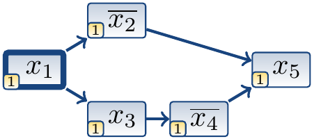
Consider again the formula \begin{eqnarray*} (\Neg{x_1} \lor \Neg{x_2}) \land (\Neg{x_1} \lor x_3) \land (\Neg{x_3} \lor \Neg{x_4}) \land (x_2 \lor x_4 \lor x_5) &\land&\\\\ (\Neg{x_5} \lor x_6 \lor \Neg{x_7}) \land (x_2 \lor x_7 \lor x_8) \land (\Neg{x_8} \lor \Neg{x_9}) \land (\Neg{x_8} \lor x_{10}) &\land&\\\\ (x_9 \lor \Neg{x_{10}} \lor x_{11}) \land (\Neg{x_{10}} \lor \Neg{x_{12}}) \land (\Neg{x_{11}} \lor x_{12}). \end{eqnarray*} As we saw in the previous example, after deciding that \( x_1 \) is true, the trail is \( \Anno{x_1}{\Dec}\ \Anno{\Neg{x_2}}{(\Neg{x_1} \lor \Neg{x_2})}\ \Anno{x_3}{(\Neg{x_1} \lor x_3)}\ \Anno{\Neg{x_4}}{(\Neg{x_3} \lor \Neg{x_4})}\ \Anno{x_5}{(x_2 \lor x_4 \lor x_5)} \). The corresponding implication graph is shown below. For convenience only, the decision literal vertex is drawn with thick lines and the decision level is marked in each vertex.

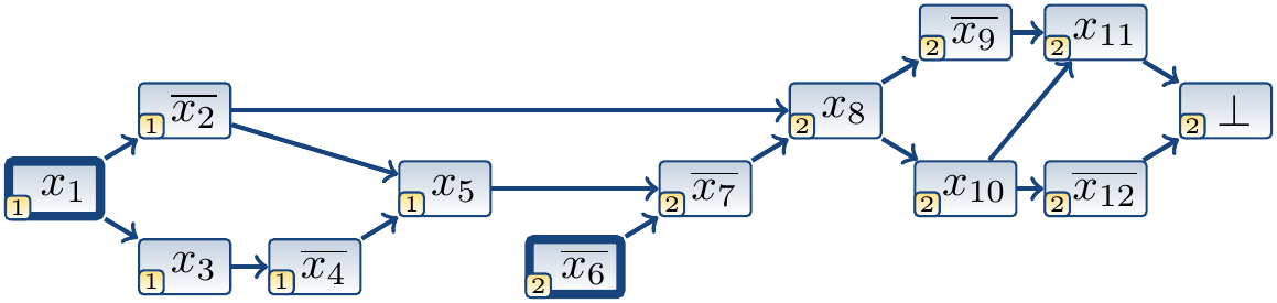
After deciding that \( x_6 \) is false, the trail is \[\Anno{x_1}{\Dec}\ \Anno{\Neg{x_2}}{(\Neg{x_1} \lor \Neg{x_2})}\ \Anno{x_3}{(\Neg{x_1} \lor x_3)}\ \Anno{\Neg{x_4}}{(\Neg{x_3} \lor \Neg{x_4})}\ \Anno{x_5}{(x_2 \lor x_4 \lor x_5)}\\\\ \Anno{\Neg{x_6}}{\Dec} \Anno{\Neg{x_7}}{(\Neg{x_5} \lor x_6 \lor \Neg{x_7})} \Anno{x_8}{(x_2 \lor x_7 \lor x_8)} \Anno{\Neg{x_9}}{(\Neg{x_8} \lor \Neg{x_9})} \Anno{x_{10}}{(\Neg{x_8} \lor x_{10})} \Anno{x_{11}}{(x_9 \lor \Neg{x_{10}} \lor x_{11})} \Anno{\Neg{x_{12}}}{(\Neg{x_{10}} \lor \Neg{x_{12}})}\] and the corresponding implication graph is shown below. Observe the conflict vertex \( \IGConflict \) whose incoming edges originate from the negations of the literals of the falsified clause \( (\Neg{x_{11}} \lor x_{12}) \).

The implication graphs allow us to define possible reasons for a conflict. The idea is to pick a subset of the literals in the graph such that by using unit clause propagation only, the same conflict can be obtained. The learned clause is then simply the clause that forbids this set of literals from appearing again in the search.

Definition: Conflict cuts and learned clauses

Consider an implication graph \( \Pair{\IGVerts}{\IGEdges} \) obtained from a trail that falsifies at least one clause. A conflict cut of the graph is a partition \( W = \Pair{A}{B} \) of its vertex set such that

all the decision literal vertices belong to the set \( A \), and
the conflict vertex \( \IGConflict \) belongs to the set \( B \).

Let \( R = \Setdef{l \in A}{\exists l’ \in B: \IGEdge{l}{l’} \in \IGEdges} \) be the reason set of the conflict cut consisting of the \( A \)-vertices having an edge to the \( B \) set.

The learned clause corresponding to the cut is \( \bigvee_{l \in R}\Neg{l} \).

Observe the following:

Setting all \( R \)-literals to true and performing unit propagation will produce a conflict.
Therefore \( \phi \Models \neg (\bigwedge_{l \in R} l) \) and thus the learned clause \( \bigvee_{l \in R}\Neg{l} \) is a logical consequence of \( \phi \).

As a consequence, adding learned clauses to the CNF formula \( \phi \) will preserve all its satisfying truth assignments.

Example

Consider again the implication graph of the previous example, shown below.

Let’s next see some possible conflicts cuts and learned clauses on it.

In the cut below, we have that \( A = \Set{x_1,\Neg{x_6}} \), \( R = \Set{x_1,\Neg{x_6}} \), and the learned clause is \( (\Neg{x_1} \lor x_6) \).
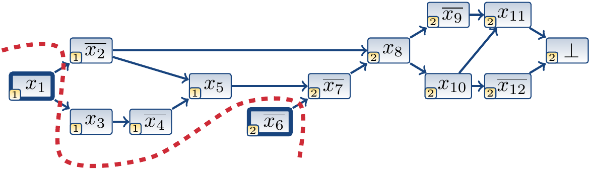
In the cut below, we have that \( A = \Set{x_1,\Neg{x_2},x_3,\Neg{x_4},x_5,\Neg{x_6}} \), \( R = \Set{\Neg{x_2},x_5,\Neg{x_6}} \), and the learned clause \( (x_2 \lor \Neg{x_5} \lor x_6) \).
In the cut below, we have that \( A = \Set{x_1,…,\Neg{x_7},x_8} \), \( R = \Set{x_8} \), and the learned clause \( (\Neg{x_8}) \).
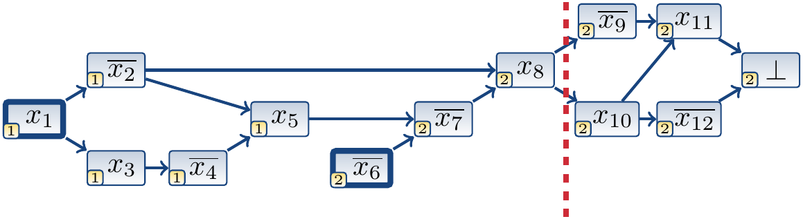
In the cut below, we have that \( A = \Set{x_1,…,x_5,\Neg{x_6},x_{10}} \), \( R = \Set{\Neg{x_2},x_5,\Neg{x_6},x_{10}} \), and the learned clause \( (x_2 \lor \Neg{x_5} \lor x_6 \lor \Neg{x_{10}}) \).

In practise, we only consider certain cuts that have some special properties. Especially, as we use unit propagation as the constraint propagation engine, learned clauses should enable new unit propagation steps.

Definition: Unique implication points and UIP cuts

A vertex \( l \) in the implication graph is a unique implication point (UIP) if all the paths from the latest decision literal vertex to the conflict vertex go through \( l \).

If \( l \) is a UIP, then the corresponding UIP cut is \( (A,B) \), where \( B \) contains all the successors of \( l \) from which there is a path to \( \IGConflict \) and \( A \) contains the rest.

Observe that UIP cuts always exist: the latest decision vertex is a UIP by definition. Especially, we use the first UIP cut: the UIP cut with the largest possible \( A \) set.

Example

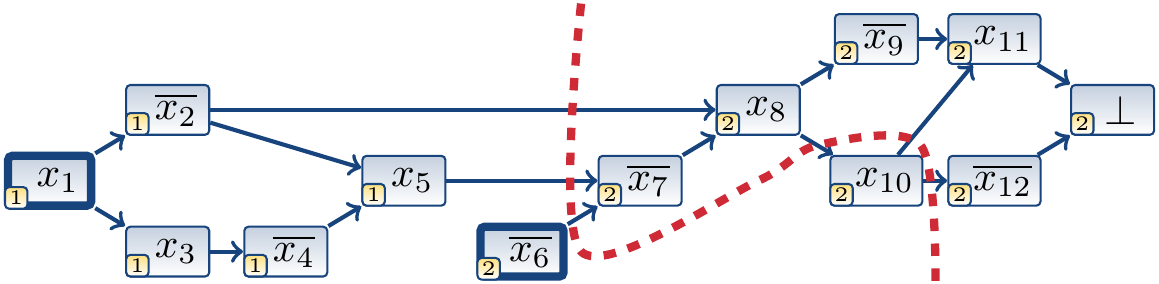
Consider again the implication graph of the previous example, shown below. It has three UIPs: \( \Neg{x_6} \), \( \Neg{x_7} \), and \( x_8 \).

The cut below is not an UIP cut as the set \( B \) contains vertices other than the successors of the UIP \( \Neg{x_6} \).
The cut below is an UIP cut but not the first UIP cut.
The cut below is an UIP cut but not the first UIP cut.
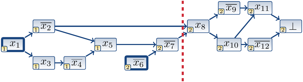
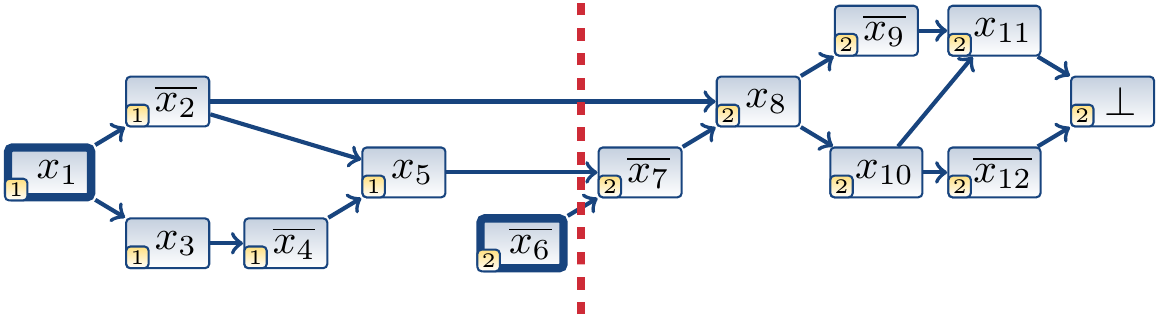
The cut below is the first UIP cut

Suppose that we take the learned clause \( C \) from an UIP cut. As we saw earlier, \( C \) is a logical consequence of \( \phi \) and we may “learn” \( C \) by adding it to \( \phi \). This preserves all the satisfying truth assignments of \( \phi \).

After learning, the CDCL algorithm now performs non-chronological backjumping:

Let \( m \) be the second largest decision level of the literals in \( C \) (or 0 if \( C \) contains only one literal).
Remove all the literals with decision level greater than \( m \) from the trail.

Because \( C \) is derived from an UIP cut, it had exactly one literal in the latest decision level before backjumping and therefore, after backjumping, \( C \) allows new unit propagation.

Example: Continued…

Consider the UIP cut below.

It produces the learned clause \( (x_2 \lor \Neg{x_5} \lor x_6) \).

After learning the clause, the CDCL algorithm backjumps to the level 1 and then unit propagates \( x_6 \) to true by using the learned clause.

The new trail is: \( \Anno{x_1}{\Dec}\ \Anno{\Neg{x_2}}{(\Neg{x_1} \lor \Neg{x_2})}\ \Anno{x_3}{(\Neg{x_1} \lor x_3)}\ \Anno{\Neg{x_4}}{(\Neg{x_3} \lor \Neg{x_4})}\ \Anno{x_5}{(x_2 \lor x_4 \lor x_5)} \Anno{x_6}{(x_2 \lor \Neg{x_5} \lor x_6)} \)
Consider the first UIP cut below.

It produces the learned clause \( (\Neg{x_8}) \).

After learning the clause, the CDCL algorithm backjumps to the level 0 and then unit propagates \( x_8 \) to false by using the learned clause.

The new trail is: \( \Anno{\Neg{x_8}}{(\Neg{x_8})} \)

The learned clauses can be seen as “lemmas” that are added to the formula and enhance the power of unit propagation. Observe that all the literals at the decision level 0 are logical consequences of the formula and thus true in all the satisfying truth assignments (thus, in practise, the negations of the decision level 0 literals are not included in the learned clauses).

For satisfiable formulas, the CDCL algorithm eventually finds a satisfying truth assignment because the learned clauses preserve them.
For unsatisfiable formulas, the algorithm eventually reports “unsatisfiable” because each conflict results in a new learned clause. There are only finitely many possible clauses and thus the algorithm will produce enough unary clauses at some point for a level 0 conflict marking unsatisfiability.

Example: A full execution of the CDCL algorithm

Consider the CNF formula \begin{eqnarray*} (a \lor b \lor c) \land (a \lor b \lor \Neg{c}) \land (\Neg{b} \lor d) &\land& \\\\ (a \lor \Neg{b} \lor \Neg{d}) \land (\Neg{a} \lor e \lor f) \land (\Neg{a} \lor e \lor \Neg{f}) &\land& \\\\ (\Neg{e} \lor \Neg{f}) \land (\Neg{a} \lor \Neg{e} \lor f) && \end{eqnarray*} One possible execution of the CDCL algorithm on it is as follows:

The formula does not contain unit clauses and thus the decision level \( 0 \) is empty in the beginning.
At the decision level 1, assume that \( a \) is false. Unit propagation does not propagate anything and the trail is thus \( \Anno{\Neg{a}}{\Dec} \).
At the decision level 2, assume that \( b \) is false. Unit propagation on the clause \( (a \lor b \lor c) \) produces the trail \( \Anno{\Neg{a}}{\Dec} \Anno{\Neg{b}}{\Dec} \Anno{c}{(a \lor b \lor c)} \). Thus a conflict is obtained as the clause \( (a \lor b \lor \Neg{c}) \) is falsified.

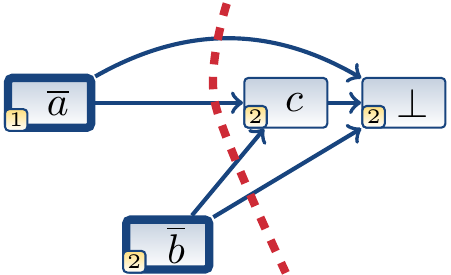
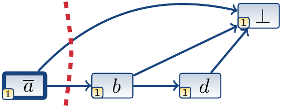
Performing conflict analysis with the 1-UIP cut produces the learned clause \( (a \lor b) \), which is included in the formula. The algorithm thus backtracks to the decision level 1.
At the decision level 1, unit propagation first deduces that \( b \) is true by using the learned clause \( (a \lor b) \), and then that \( d \) is true by using the clause \( (\Neg{b} \lor d) \). The trail is now \( \Anno{\Neg{a}}{\Dec} \Anno{b}{(a \lor b)} \Anno{d}{(\Neg{b} \lor d)} \) and a conflict occurs as the clause is \( (a \lor \Neg{b} \lor \Neg{d}) \) falsified.

Performing conflict analysis with the 1-UIP cut produces the learned clause \( (a) \), which is included in the formula. The algorithm thus backtracks to the decision level 0.
At the decision level 0, unit propagation sets \( a \) to true and the trail is \( \Anno{a}{(a)} \).
At the decision level 1, assume that \( e \) is false. Unit propagation now sets \( f \) to true by using the clause \( (\Neg{a} \lor e \lor f) \). The trail is now \( \Anno{a}{(a)} \Anno{\Neg{e}}{\Dec} \Anno{f}{(\Neg{a} \lor e \lor f)} \) and a conflict occurs as the clause \( (\Neg{a} \lor e \lor \Neg{f}) \) is falsified.

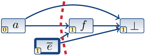
Performing conflict analysis with the 1-UIP cut produces the learned clause \( (e) \), which is included in the formula. Notice that \( \Neg{a} \) is not included in the learned clause because the literal \( a \) is at the decision level 0 and thus always true. The algorithm now backtracks to the decision level 0.
At the decision level 0, unit propagation sets \( e \) to true by using the learned unit clause \( (e) \) and then \( f \) to false by using the clause \( (\Neg{e} \lor \Neg{f}) \). The trail is \( \Anno{a}{(a)} \Anno{e}{(e)} \Anno{\Neg{f}}{(\Neg{e} \lor \Neg{f})} \) and a conflict occurs as the clause \( (\Neg{a} \lor \Neg{e} \lor f) \) is falsified.

As a conflict is obtained at the decision level 0, the algorithm terminates and reports that the formula is unsatisfiable.

Some omitted (major!) components¶

We’ve skipped several crucial parts needed to make the CDCL approach really work in practise:

Heuristics for making decisions; They usully try to select variables that occurred recently in many conflicts.
Data structures for fast unit propagation (of large learned clauses).
Forgetting learned clauses (to save memory).
Restarts (for escaping from difficult parts).
Learned clause minimization.
And so on…

Some classic references for further study:

Handbook of Satisfiability
The Chaff: Engineering an Efficient SAT Solver paper introducing data structures for fast unit propagation and the original VSIDS literal selection heuristics
The An Extensible SAT-solver paper
The source code of the MiniSat solver
The solver descriptions in the yearly SAT competitions