Post-hoc modification of linear models¶

This example will demonstrate how a simple linear decoder can be enhanced through post-hoc modification. This example contains the core ideas that are presented in the main paper 1.

We will start with a logistic regressor as a base model. Then, we will modify the covariance matrix by applying shrinkage, modify the pattern with a Gaussian kernel and modify the normalizer to be “unit noise gain”, meaning the weights all sum to 1.

Author: Marijn van Vliet <w.m.vanvliet@gmail.com>

# Required imports
import numpy as np
from scipy.stats import norm
import mne
from posthoc import Workbench, cov_estimators, normalizers
from sklearn.model_selection import StratifiedKFold
from sklearn.metrics import accuracy_score
from sklearn.linear_model import LogisticRegression
from matplotlib import pyplot as plt

We will use the MNE sample dataset. It is an MEG recording of a participant listening to auditory beeps and looking at visual stimuli. For this example, we attempt to discriminate between auditory beeps presented to the left versus the right of the head. The following code reads in the sample dataset.

path = mne.datasets.sample.data_path()
raw = mne.io.read_raw_fif(path + '/MEG/sample/sample_audvis_raw.fif',
                          preload=True)
events = mne.find_events(raw)
event_id = dict(left=1, right=2)
raw.pick_types(meg='grad')
raw.filter(None, 20)
raw, events = raw.resample(50, events=events)

# Create epochs
epochs = mne.Epochs(raw, events, event_id, tmin=-0.2, tmax=0.5,
                    baseline=(-0.2, 0), preload=True)
n_epochs, n_channels, n_samples = epochs.get_data().shape

The data is now loaded as an mne.Epochs object. In order to use the sklearn and posthoc packages effectively, we need to shape this data into a (observations x features) matrix X and corresponding (observations x targets) y matrix.

X = epochs.get_data().reshape(len(epochs), -1)

# The classification algorithm doesn't handle small values well. Convert the
# units of X into femto-Teslas
X *= 1E15

# Create training labels, based on the event codes during the experiment.
y = epochs.events[:, 2]
y = y - 1.5
y *= 2
y = y.astype(int)

Now, we are ready to define a logistic regression model and apply it to the data. We split the data 50/50 into a training and test set. We present the training data to the model to learn from and test its performance on the test set.

# Split the data 50/50, but make sure the number of left/right epochs are
# balanced.
folds = StratifiedKFold(n_splits=2)
train_index, test_index = next(folds.split(X, y))
X_train, y_train = X[train_index], y[train_index]
X_test, y_test = X[test_index], y[test_index]

# The logistic regression model ignores observations that are close to the
# decision boundary. The parameter `C` controls how far away observations have
# to be in order to not be ignored. A setting of 20 means "quite far". We also
# specify the seed for the random number generator, so that this example
# replicates exactly every time.
base_model = LogisticRegression(C=20, solver='lbfgs', random_state=0)

# Train on the training data and predict the test data.
base_model.fit(X_train, y_train)
y_hat = base_model.predict(X_test)

# How many epochs did we decode correctly?
base_model_accuracy = accuracy_score(y_test, y_hat)
print('Base model accuracy: %.2f%%' % (100 * base_model_accuracy))

Out:

Base model accuracy: 73.97%

To inspect the pattern that the model has learned, we wrap the model in a posthoc.Workbench object. After fitting, this object exposes the .pattern_ attribute.

pattern = Workbench(base_model).fit(X_train, y_train).pattern_

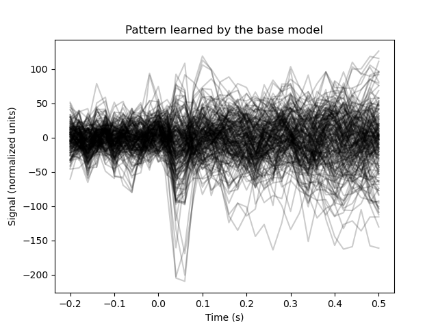
# Plot the pattern
plt.figure()
plt.plot(epochs.times, pattern.reshape(n_channels, n_samples).T,
         color='black', alpha=0.2)
plt.xlabel('Time (s)')
plt.ylabel('Signal (normalized units)')
plt.title('Pattern learned by the base model')

Out:

Text(0.5, 1.0, 'Pattern learned by the base model')

Post-hoc modification can be used to improve the model somewhat.

For starters, the template is quite noisy. The main distinctive feature between the conditions should be the auditory evoked potential around 0.05 seconds. Let’s apply post-hoc modification to inform the model of this, by multiplying the pattern with a Gaussian kernel to restrict it to a specific time interval.

# This is the Gaussian kernel we'll use
kernel = norm(13, 2).pdf(np.arange(n_samples))
kernel /= kernel.max()

# The function that modifies the pattern takes as input the original pattern
# and the training data.
def pattern_modifier(pattern, X, y):
    """Multiply the pattern with a Gaussian kernel."""
    mod_pattern = pattern.reshape(n_channels, n_samples)
    mod_pattern = mod_pattern * kernel[np.newaxis, :]
    return mod_pattern.reshape(pattern.shape)

Now we can assemble the post-hoc model. The covariance matrix is computed using a shrinkage estimator. Since the number of features far exceeds the number of training observations, the kernel version of the estimator is much faster. We modify the pattern using the pattern_modifier function that we defined earlier, but modifying the pattern like this will affect the scaling of the output. To obtain a result with a consistent scaling, we modify the normalizer such that the modified pattern passes through our model with unit gain.

# Define the post-hoc model
optimized_model = Workbench(
    base_model,
    cov=cov_estimators.ShrinkageKernel(1.0),
    pattern_modifier=pattern_modifier,
    normalizer_modifier=normalizers.unit_gain,
).fit(X_train, y_train)

# Decode the test data
y_hat = optimized_model.predict(X_test).ravel()

# Assign the 'left' class to values above 0 and 'right' to values below 0
y_bin = np.zeros(len(y_hat), dtype=np.int)
y_bin[y_hat >= 0] = 1
y_bin[y_hat < 0] = -1

# How many epochs did we decode correctly?
optimized_model_accuracy = accuracy_score(y_test, y_bin)
print('Base model accuracy: %.2f%%' % (100 * base_model_accuracy))
print('Optimized model accuracy: %.2f%%' % (100 * optimized_model_accuracy))

Out:

Base model accuracy: 73.97%
Optimized model accuracy: 84.93%

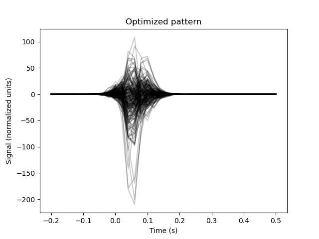
The post-hoc model performs better. Let’s visualize the optimized pattern.

plt.figure()
plt.plot(epochs.times,
         optimized_model.pattern_.reshape(n_channels, n_samples).T,
         color='black', alpha=0.2)
plt.xlabel('Time (s)')
plt.ylabel('Signal (normalized units)')
plt.title('Optimized pattern')

Out:

Text(0.5, 1.0, 'Optimized pattern')

References¶

1: Marijn van Vliet and Riitta Salmelin (2020). Post-hoc modification of linear models: combining machine learning with domain information to make solid inferences from noisy data. Neuroimage, 204, 116221. https://doi.org/10.1016/j.neuroimage.2019.116221

sphinx_gallery_thumbnail_number = 2

Total running time of the script: ( 0 minutes 15.363 seconds)

Download Python source code: plot_post_hoc.py

Download Jupyter notebook: plot_post_hoc.ipynb

Gallery generated by Sphinx-Gallery