Decoding with a spatio-temporal LCMV beamformer¶

This example will demonstrate a simple decoder based on an LCMV beamformer applied to the MNE-Sample dataset. This dataset contains MEG recordings of a subject being presented with audio beeps on either the left or right side of the head.

This approach is further documented in van Vliet et al. 2016 1.

First, some required Python modules and loading the data:

import numpy as np
import mne
from posthoc import Beamformer
from posthoc.cov_estimators import ShrinkageKernel
from sklearn.model_selection import StratifiedKFold
from sklearn import metrics
from matplotlib import pyplot as plt

mne.set_log_level(False)  # Be very very quiet

path = mne.datasets.sample.data_path()
raw = mne.io.read_raw_fif(path + '/MEG/sample/sample_audvis_raw.fif',
                          preload=True)
events = mne.find_events(raw)
event_id = dict(left=1, right=2)
raw.pick_types(meg='grad')
raw.filter(None, 20)
raw, events = raw.resample(50, events=events)

epochs = mne.Epochs(raw, events, event_id, tmin=-0.2, tmax=0.5,
                    baseline=(-0.2, 0), preload=True)

The post-hoc package uses a scikit-learn style API. We must translate the MNE-Python epochs object into scikit-learn style X and y matrices.

X = epochs.get_data().reshape(len(epochs), -1)
y = epochs.events[:, 2]

# Split the data in a train and test set
folds = StratifiedKFold(n_splits=2)
train_index, test_index = next(folds.split(X, y))
X_train, y_train = X[train_index], y[train_index]
X_test, y_test = X[test_index], y[test_index]

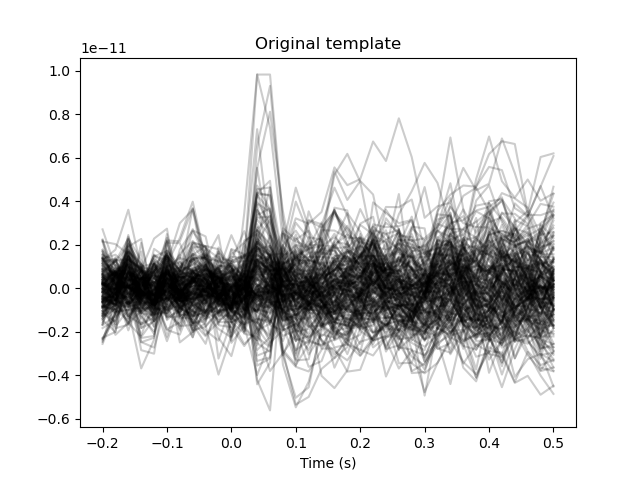
We will now use some of the epochs to construct a template of the difference between the ‘left’ and ‘right’ reponses. For this, we compute the “evoked potential” for the left and right beeps. The contrast between these conditions will serve as our template. This template is then further refined with a Hanning window to focus on a specific part of the evoked potential.

evoked_left = X_train[y_train == 1].mean(axis=0)
evoked_right = X_train[y_train == 2].mean(axis=0)
template = evoked_left - evoked_right

# This creates a (channels x time) view of the template
template_ch_time = template.reshape(epochs.info['nchan'], -1)

# Plot the template
plt.figure()
plt.plot(epochs.times, template_ch_time.T, color='black', alpha=0.2)
plt.xlabel('Time (s)')
plt.title('Original template')

Out:

Text(0.5, 1.0, 'Original template')

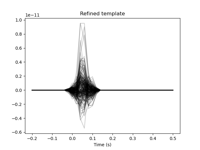
The template is quite noisy. The main distinctive feature between the conditions should be the auditory evoked potential around 0.05 seconds. Let’s create a Hanning window to limit our template to just the evoked potential.

center = np.searchsorted(epochs.times, 0.05)
width = 10
window = np.zeros(len(epochs.times))
window[center - width // 2: center + width // 2] = np.hanning(width)
template_ch_time *= window[np.newaxis, :]

# Plot the refined template
plt.figure()
plt.plot(epochs.times, template_ch_time.T, color='black', alpha=0.2)
plt.xlabel('Time (s)')
plt.title('Refined template')

Out:

Text(0.5, 1.0, 'Refined template')

Now, we make an LCMV beamformer based on the template. We apply heavy shrinkage regularization to the covariance matrix to deal with the fact that we have so few trials and a huge number of features: (203 channels x 50 time points = 7308)

beamformer = Beamformer(template, cov=ShrinkageKernel(1.0)).fit(X_train)

# Decode the test data
y_hat = beamformer.predict(X_test).ravel()

# Visualize the output of the LCMV beamformer
y_left = y_hat[y_test == 1]
y_right = y_hat[y_test == 2]
lim = np.max(np.abs(y_hat))
plt.figure()
plt.scatter(np.arange(len(y_left)), y_left)
plt.scatter(np.arange(len(y_left), len(y_left) + len(y_right)), y_right)
plt.legend(['left', 'right'])
plt.axhline(0, color='gray')
plt.ylim(-lim, lim)
plt.xlabel('Epochs')
plt.ylabel('Beamformer output')

# Assign the 'left' class to values above 0 and 'right' to values below 0
y_bin = np.zeros(len(y_hat), dtype=np.int)
y_bin[y_hat >= 0] = 1
y_bin[y_hat < 0] = 2

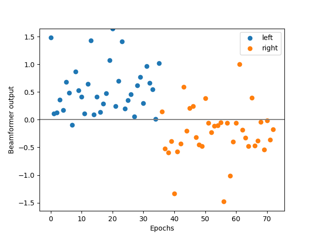
So, how did we do? What percentage of the epochs did we decode correctly?

print('LCMV accuracy: %.2f%%' % (100 * metrics.accuracy_score(y_test, y_bin)))

Out:

LCMV accuracy: 89.04%

References¶

1: van Vliet, M., Chumerin, N., De Deyne, S., Wiersema, J. R., Fias, W., Storms, G., & Van Hulle, M. M. (2016). Single-trial ERP component analysis using a spatiotemporal LCMV beamformer. IEEE Transactions on Biomedical Engineering, 63(1), 55–66. https://doi.org/10.1109/TBME.2015.2468588

Total running time of the script: ( 0 minutes 6.119 seconds)

Gallery generated by Sphinx-Gallery