Plot sensor-level RDMs

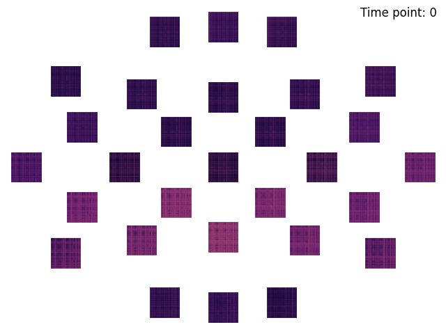
This example demonstrates how to visualize representational dissimilarity matrices (RDMs) computed from EEG data. We will compute them using a spatial searchlight and plot the RDM computed for each searchlight-patch.

# Import required packages
import numpy as np
import mne
import mne_rsa

MNE-Python contains a build-in data loader for the kiloword dataset. We use it here to read it as 960 epochs. Each epoch represents the brain response to a single word, averaged across all the participants. For this example, we speed up the computation, at a cost of temporal precision, by downsampling the data from the original 250 Hz. to 100 Hz.

data_path = mne.datasets.kiloword.data_path(verbose=True)
epochs = mne.read_epochs(data_path / "kword_metadata-epo.fif")
epochs = epochs.resample(100)

Reading C:\Users\wmvan\mne_data\MNE-kiloword-data\kword_metadata-epo.fif ...
Isotrak not found
    Found the data of interest:
        t =    -100.00 ...     920.00 ms
        0 CTF compensation matrices available
Adding metadata with 8 columns
960 matching events found
No baseline correction applied
0 projection items activated

We now compute RDMs using a spatial searchlight with a radius of 45 centimeters.

# This will create a generator for the RDMs
rdms = mne_rsa.rdm_epochs(
    epochs,  # The EEG data
    dist_metric="correlation",  # Metric to compute the EEG RDMs
    spatial_radius=45,  # Spatial radius of the searchlight patch
    temporal_radius=None,  # Perform only spatial searchlight
    tmin=0.15,
    tmax=0.25,  # To save time, only analyze this time interval
)

# Unpack the generator into a NumPy array so we can plot it
rdms = np.array(list(rdms))

# Visualize the RDMs.
mne_rsa.viz.plot_rdms_topo(rdms, epochs.info, cmap="magma")

Creating spatial searchlight patches

<Figure size 640x480 with 29 Axes>