Note
Go to the end to download the full example code.
Sensor-level RSA using a searchlight#
This example demonstrates how to perform representational similarity analysis (RSA) on EEG data, using a searchlight approach.
In the searchlight approach, representational similarity is computed between the model and searchlight “patches”. A patch is defined by a seed point (e.g. sensor Pz) and everything within the given radius (e.g. all sensors within 4 cm. of Pz). Patches are created for all possible seed points (e.g. all sensors), so you can think of it as a “searchlight” that moves from seed point to seed point and everything that is in the spotlight is used in the computation.
The radius of a searchlight can be defined in space, in time, or both. In this example, our searchlight will have a spatial radius of 4.5 cm. and a temporal radius of 50 ms.
- ..warning::
A searchlight across MEG sensors does not make a lot of sense, as the magnetic field pattern does not lend itself well to circular searchlight patches.
The dataset will be the kiloword dataset [1]: approximately 1,000 words were presented to 75 participants in a go/no-go lexical decision task while event-related potentials (ERPs) were recorded.
Authors#
Marijn van Vliet <marijn.vanvliet@aalto.fi>
# sphinx_gallery_thumbnail_number=2

# Import required packages
import mne
import mne_rsa
MNE-Python contains a build-in data loader for the kiloword dataset. We use it here to read it as 960 epochs. Each epoch represents the brain response to a single word, averaged across all the participants. For this example, we speed up the computation, at a cost of temporal precision, by downsampling the data from the original 250 Hz. to 100 Hz.
data_path = mne.datasets.kiloword.data_path(verbose=True)
epochs = mne.read_epochs(data_path / "kword_metadata-epo.fif")
epochs = epochs.resample(100)
The kiloword datas was erroneously stored with sensor locations given in centimeters instead of meters. We will fix it now. For your own data, the sensor locations are likely properly stored in meters, so you can skip this step.
for ch in epochs.info["chs"]:
    ch["loc"] /= 100
The epochs object contains a .metadata field that contains information about
the 960 words that were used in the experiment. Let’s have a look at the metadata for
10 random words:
epochs.metadata.sample(10)
Let’s pick something obvious for this example and build a dissimilarity matrix (RDM) based on the number of letters in each word.
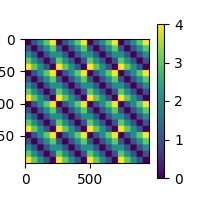
<Figure size 200x200 with 2 Axes>
The above RDM will serve as our “model” RDM. In this example RSA analysis, we are going to compare the model RDM against RDMs created from the EEG data. The EEG RDMs will be created using a “searchlight” pattern. We are using squared Euclidean distance for our RDM metric, since we only have a few data points in each searchlight patch. Feel free to play around with other metrics.
rsa_result = mne_rsa.rsa_epochs(
    epochs,  # The EEG data
    rdm_vis,  # The model RDM
    epochs_rdm_metric="sqeuclidean",  # Metric to compute the EEG RDMs
    rsa_metric="kendall-tau-a",  # Metric to compare model and EEG RDMs
    spatial_radius=0.05,  # Spatial radius of the searchlight patch in meters.
    temporal_radius=0.05,  # Temporal radius of the searchlight path in seconds.
    tmin=0.15,
    tmax=0.25,  # To save time, only analyze this time interval
    n_jobs=1,  # Only use one CPU core. Increase this for more speed.
    n_folds=None,  # Don't use any cross-validation
    verbose=False,
)  # Set to True to display a progress bar
The result is packed inside an MNE-Python mne.Evoked object. This object
defines many plotting functions, for example mne.Evoked.plot_topomap() to look
at the spatial distribution of the RSA values. By default, the signal is assumed to
represent micro-Volts, so we need to explicitly inform the plotting function we are
plotting RSA values and tweak the range of the colormap.
rsa_result.plot_topomap(
    rsa_result.times,
    units=dict(eeg="kendall-tau-a"),
    scalings=dict(eeg=1),
    cbar_fmt="%.4f",
    vlim=(0, None),
    nrows=2,
    sphere=1,
)
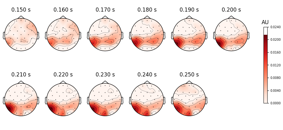
<MNEFigure size 900x415 with 12 Axes>
Unsurprisingly, we get the highest correspondance between number of letters and EEG signal in areas in the visual word form area.
Total running time of the script: (0 minutes 58.675 seconds)