Source-level RSA using a searchlight on fMRI data

This example demonstrates how to perform representational similarity analysis (RSA) on volumetric fMRI data, using a searchlight approach.

In the searchlight approach, representational similarity is computed between the model and searchlight “patches”. A patch is defined by a seed voxel and all voxels within a given radius. By default, patches are created using each voxel as a seed point, so you can think of it as a “searchlight” that scans through the brain. In this example, our searchlight will have a spatial radius of 1 cm.

The dataset will be the Haxby et al. 2001 dataset: a collection of 1452 scans during which the participant was presented with a stimulus image belonging to any of 8 different classes: scissors, face, cat, shoe, house, scrambledpix, bottle, chair.

# sphinx_gallery_thumbnail_number=2

# Import required packages
import mne_rsa
import nibabel as nib
import pandas as pd
import tarfile
import urllib.request
from nilearn.plotting import plot_glass_brain

We’ll be using the data from the Haxby et al. 2001 set, which can be found at: http://data.pymvpa.org/datasets/haxby2001

# Download and extract data
fname, _ = urllib.request.urlretrieve(
    "http://data.pymvpa.org/datasets/haxby2001/subj1-2010.01.14.tar.gz"
)
tar = tarfile.open(fname, "r:gz")
tar.extractall()
tar.close()

# Load fMRI BOLD data
bold = nib.load("subj1/bold.nii.gz")

# This is a mask that the authors provide. It is a GLM contrast based
# localizer map that extracts an ROI in the "ventral temporal" region.
mask = nib.load("subj1/mask4_vt.nii.gz")

# This is the metadata of the experiment. What stimulus was shown when etc.
meta = pd.read_csv("subj1/labels.txt", sep=" ")
meta["labels"] = meta["labels"].astype("category")

Drop “rest” class and sort images by class. We must ensure that all times, the metadata and the bold images are in sync. Hence, we first perform the operations on the meta pandas DataFrame. Then, we can use the DataFrame’s index to repeat the operations on the BOLD data.

meta = meta[meta["labels"] != "rest"].sort_values("labels")
bold = nib.Nifti1Image(bold.get_fdata()[..., meta.index], bold.affine, bold.header)

We’re going to hunt for areas in the brain where the signal differentiates nicely between the various object categories. We encode this objective in our “model” RDM: a RDM where stimuli belonging to the same object category have a dissimilarity of 0 and stimuli belonging to different categories have a dissimilarity of 1.

model_rdm = mne_rsa.compute_rdm(meta["labels"], metric=lambda a, b: 0 if a == b else 1)
mne_rsa.plot_rdms(model_rdm, "Model RDM")

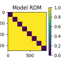
<Figure size 200x200 with 2 Axes>

Performing the RSA. This will take some time. Consider increasing n_jobs to parallelize the computation across multiple CPUs.

rsa_vals = mne_rsa.rsa_nifti(
    bold,  # The BOLD data
    model_rdm,  # The model RDM we constructed above
    image_rdm_metric="correlation",  # Metric to compute the BOLD RDMs
    rsa_metric="kendall-tau-a",  # Metric to compare model and BOLD RDMs
    spatial_radius=0.01,  # Spatial radius of the searchlight patch
    roi_mask=mask,  # Restrict analysis to the VT ROI
    n_jobs=1,  # Only use one CPU core.
    verbose=False,
)  # Set to True to display a progress bar

Plot the result using nilearn.

plot_glass_brain(rsa_vals)

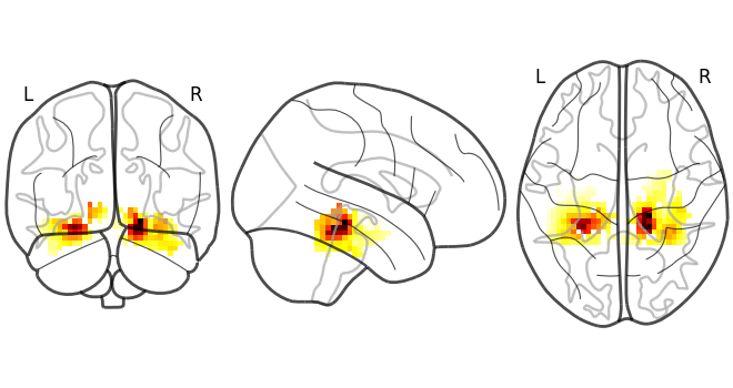
<nilearn.plotting.displays._projectors.OrthoProjector object at 0x000002B7A0C28BB0>