DICS for power mapping and connectivity analysis

In this tutorial, we’re going to simulate two signals originating from two locations on the cortex. These signals will be sine waves, so we’ll be looking at oscillatory activity (as opposed to evoked activity). These signals will also be coherent, which means they are correlated in the frequency domain. Coherence is thought to be indicative of communication between brain areas and can be used as a measure of functional connectivity [1]. So we are effectively simulating two active brain regions that communicate with each-other.

We’ll be using dynamic imaging of coherent sources (DICS) [2] to map out all-to-all functional connectivity between brain regions. Let’s see if we can find our two simulated coherent sources.

This tutorial aims to give you an introduction to function connectivity analysis on a toy dataset. Analyzing a real dataset entails many methodological considerations, which are discussed in [3].

# Author: Marijn van Vliet <w.m.vanvliet@gmail.com>
#
# License: BSD (3-clause)

Setup

We first import the required packages to run this tutorial and define a list of filenames for various things we’ll be using.

import os.path as op
import numpy as np
from scipy.signal import welch, coherence
from matplotlib import pyplot as plt

# The conpy package implements DICS connectivity
from conpy import (
    dics_connectivity,
    all_to_all_connectivity_pairs,
    one_to_all_connectivity_pairs,
    forward_to_tangential,
)

# MNE implements all other EEG analysis tools.
import mne
from mne.datasets import sample, testing
from mne.minimum_norm import make_inverse_operator, apply_inverse
from mne.time_frequency import csd_morlet
from mne.beamformer import make_dics, apply_dics_csd

# Suppress irrelevant output
mne.set_log_level("ERROR")

# We use the MEG and MRI setup from the MNE-sample dataset
data_path = sample.data_path(download=True)
subjects_dir = op.join(data_path, "subjects")
mri_path = op.join(subjects_dir, "sample")

# Filenames for various files we'll be using
meg_path = op.join(data_path, "MEG", "sample")
trans_fname = op.join(meg_path, "sample_audvis_raw-trans.fif")
fwd_fname = op.join(meg_path, "sample_audvis-meg-eeg-oct-6-fwd.fif")

# Later on, we'll use the forward model defined in the MNE-testing dataset
testing_path = op.join(testing.data_path(download=True), "MEG", "sample")
fwd_lim_fname = op.join(testing_path, "sample_audvis_trunc-meg-eeg-oct-4-fwd.fif")

# Seed for the random number generator
np.random.seed(42)

Data simulation

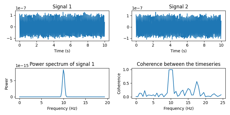
The following function generates a timeseries that contains an oscillator, whose frequency fluctuates a little over time, but stays close to 10 Hz. We’ll use this function to generate our two signals.

sfreq = 50  # Sampling frequency of the generated signal
times = np.arange(10.0 * sfreq) / sfreq  # 10 seconds of signal


def coh_signal_gen():
    """Generate an oscillating signal.

    Returns
    -------
    signal : ndarray
        The generated signal.
    """
    t_rand = 0.001  # Variation in the instantaneous frequency of the signal
    std = 0.1  # Std-dev of the random fluctuations added to the signal
    base_freq = 10.0  # Base frequency of the oscillators in Hertz
    n_times = len(times)

    # Generate an oscillator with varying frequency and phase lag.
    iflaw = base_freq / sfreq + t_rand * np.random.randn(n_times)
    signal = np.exp(1j * 2.0 * np.pi * np.cumsum(iflaw))
    signal *= np.conj(signal[0])
    signal = signal.real

    # Add some random fluctuations to the signal.
    signal += std * np.random.randn(n_times)
    signal *= 1e-7

    return signal

Let’s simulate two timeseries and plot some basic information about them.

signal1 = coh_signal_gen()
signal2 = coh_signal_gen()

plt.figure(figsize=(8, 4))

# Plot the timeseries
plt.subplot(221)
plt.plot(times, signal1)
plt.xlabel("Time (s)")
plt.title("Signal 1")
plt.subplot(222)
plt.plot(times, signal2)
plt.xlabel("Time (s)")
plt.title("Signal 2")

# Power spectrum of the first timeseries
f, p = welch(signal1, fs=sfreq, nperseg=128, nfft=256)
plt.subplot(223)
plt.plot(f[:100], p[:100])  # Only plot the first 30 frequencies
plt.xlabel("Frequency (Hz)")
plt.ylabel("Power")
plt.title("Power spectrum of signal 1")

# Compute the coherence between the two timeseries
f, coh = coherence(signal1, signal2, fs=sfreq, nperseg=100, noverlap=64)
plt.subplot(224)
plt.plot(f[:50], coh[:50])
plt.xlabel("Frequency (Hz)")
plt.ylabel("Coherence")
plt.title("Coherence between the timeseries")

plt.tight_layout()

Now we put the signals at two locations on the cortex. We construct a mne.SourceEstimate object to store them in.

# The locations on the cortex where the signal will originate from. These
# locations are indicated as vertex numbers.
source_vert1 = 146374
source_vert2 = 33830

# Construct a SourceEstimate object that describes the signal at the cortical
# level.
stc = mne.SourceEstimate(
    np.vstack((signal1, signal2)),  # The two signals
    vertices=[[source_vert1], [source_vert2]],  # Their locations
    tmin=0,
    tstep=1.0 / sfreq,
    subject="sample",  # We use the brain model of the MNE-Sample dataset
)

Before we simulate the sensor-level data, let’s define a signal-to-noise ratio. You are encouraged to play with this parameter and see the effect of noise on our results.

SNR = 5  # Signal-to-noise ratio. Decrease to add more noise.

Now we run the signal through the forward model to obtain simulated sensor data. To save computation time, we’ll only simulate gradiometer data. You can try simulating other types of sensors as well.

# Load the forward model
fwd = mne.read_forward_solution(fwd_fname)

# Use only gradiometers
fwd = mne.pick_types_forward(fwd, meg="grad", eeg=False, exclude="bads")

# Create an info object that holds information about the sensors (their
# location, etc.).
info = mne.create_info(fwd["info"]["ch_names"], sfreq, ch_types="grad")
with info._unlock():
    info.update(fwd["info"])

# To simulate the data, we need a version of the forward solution where each
# source has a "fixed" orientation, i.e. pointing orthogonally to the surface
# of the cortex.
fwd_fixed = mne.convert_forward_solution(fwd, force_fixed=True)

# Now we can run our simulated signal through the forward model, obtaining
# simulated sensor data.
sensor_data = mne.apply_forward_raw(fwd_fixed, stc, info).get_data()

# We're going to add some noise to the sensor data
noise = np.random.randn(*sensor_data.shape)

# Scale the noise to be in the ballpark of MEG data
noise_scaling = np.linalg.norm(sensor_data) / np.linalg.norm(noise)
noise *= noise_scaling

# Mix noise and signal with the given signal-to-noise ratio.
sensor_data = SNR * sensor_data + noise

We create an mne.EpochsArray object containing two trials: one with just noise and one with both noise and signal. The techniques we’ll be using in this tutorial depend on being able to contrast data that contains the signal of interest versus data that does not.

epochs = mne.EpochsArray(
    data=np.concatenate(
        (noise[np.newaxis, :, :], sensor_data[np.newaxis, :, :]), axis=0
    ),
    info=info,
    events=np.array([[0, 0, 1], [10, 0, 2]]),
    event_id=dict(noise=1, signal=2),
)

# Plot the simulated data
# epochs.plot()

Power mapping

With our simulated dataset ready, we can now pretend to be researchers that have just recorded this from a real subject and are going to study what parts of the brain communicate with each other.

First, we’ll create a source estimate of the MEG data. We’ll use both a straightforward MNE-dSPM inverse solution for this, and the DICS beamformer which is specifically designed to work with oscillatory data.

Computing the inverse using MNE-dSPM:

# Estimating the noise covariance on the trial that only contains noise.
cov = mne.compute_covariance(epochs["noise"])
inv = make_inverse_operator(epochs.info, fwd, cov)

# Apply the inverse model to the trial that also contains the signal.
s = apply_inverse(epochs["signal"].average(), inv)

# Take the root-mean square along the time dimension and plot the result.
s_rms = (s**2).mean()
brain = s_rms.plot(
    "sample",
    subjects_dir=subjects_dir,
    hemi="both",
    figure=1,
    time_viewer=False,
    size=400,
    title="MNE-dSPM inverse (RMS)",
)

# Indicate the true locations of the source activity on the plot.
brain.add_foci(source_vert1, coords_as_verts=True, hemi="lh")
brain.add_foci(source_vert2, coords_as_verts=True, hemi="rh")

# Rotate the view and add a title.
brain.show_view(azimuth=0, elevation=0, distance=550, focalpoint=(0, 0, 0))

fmax=1251.2662266497941
fmax=1251.2662266497941

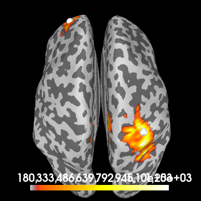
Computing a cortical power map at 10 Hz. using a DICS beamformer:

# Estimate the cross-spectral density (CSD) matrix on the trial containing the
# signal.
csd_signal = csd_morlet(epochs["signal"], frequencies=[10])

# Compute the DICS powermap.
filters = make_dics(
    epochs.info, fwd, csd_signal, inversion="single", pick_ori="max-power"
)
power, f = apply_dics_csd(csd_signal, filters)

# Plot the DICS power map.
brain = power.plot(
    "sample",
    subjects_dir=subjects_dir,
    hemi="both",
    figure=2,
    time_viewer=False,
    size=400,
    title=f"DICS power map at {f[0]:.1f} Hz",
)

# Indicate the true locations of the source activity on the plot.
brain.add_foci(source_vert1, coords_as_verts=True, hemi="lh")
brain.add_foci(source_vert2, coords_as_verts=True, hemi="rh")

# Rotate the view and add a title.
brain.show_view(azimuth=0, elevation=0, distance=550, focalpoint=(0, 0, 0))

fmax=3.549984838807983e-23
fmax=3.549984838807983e-23

Excellent! Both methods found our two simulated sources. Of course, with a signal-to-noise ratio (SNR) of 1, it isn’t very hard to find them. You can try playing with the SNR and see how the MNE-dSPM and DICS results hold up in the presense of increasing noise.

One-to-all connectivity

Let’s try to estimate coherence between the two sources. One way to do it is to compute “one-to-all” connectivity. We pick one point on the cortex where we know (or assume) that there is an active source. Then, we compute coherence between all points on the cortex and this reference point to see which parts of the cortex have a signal that is coherent with our reference source. Hopefully, we’ll find the other source.

# Our reference point is the point with maximum power (roughly the location of
# our second simulated source signal).
ref_point = np.argmax(power.data)

# Compute one-to-all coherence between each point and the reference point.
pairs = one_to_all_connectivity_pairs(fwd, ref_point)
fwd_tan = forward_to_tangential(fwd)
con = dics_connectivity(pairs, fwd_tan, csd_signal, reg=1)

To plot the result, we transform the conpy.VertexConnectivity object to an mne.SourceEstimate object, where the “signal” at each point is the coherence value.

one_to_all = con.make_stc("sum", weight_by_degree=True)

# Plot the coherence values on the cortex
brain = one_to_all.plot(
    "sample",
    subjects_dir=subjects_dir,
    hemi="both",
    figure=3,
    size=400,
    time_viewer=False,
    title="One-to-all coherence",
)

# Indicate the true locations of the source activity on the plot (in white)
brain.add_foci(source_vert1, coords_as_verts=True, hemi="lh")
brain.add_foci(source_vert2, coords_as_verts=True, hemi="rh")

# Also indicate our chosen reference point (in red). First, we need to figure
# out the vertex number of the point.
n_lh_verts = len(power.vertices[0])
if ref_point < n_lh_verts:
    hemi = "lh"
    ref_vert = power.vertices[0][ref_point]
else:
    hemi = "rh"
    ref_vert = power.vertices[1][ref_point - n_lh_verts]
brain.add_foci(ref_vert, coords_as_verts=True, hemi=hemi, color=(1, 0, 0))

# Rotate the view
brain.show_view(azimuth=0, elevation=0, distance=550, focalpoint=(0, 0, 0))

fmax=0.9763595092505787
fmax=0.9763595092505787

We see a lot of coherence in the neighbourhood surrounding the reference point, but importantly, also a local maximum in the coherence at the first source point.

Now, look what happens when we do the coherence computation again, but this time we use the trial that contains only noise.

csd_noise = csd_morlet(epochs["noise"], frequencies=[10])
con_noise = dics_connectivity(pairs, fwd_tan, csd_noise, reg=1)
one_to_all_noise = con_noise.make_stc("sum", weight_by_degree=True)

# Plot the coherence values on the cortex
brain = one_to_all_noise.plot(
    "sample",
    subjects_dir=subjects_dir,
    hemi="both",
    figure=4,
    size=400,
    time_viewer=False,
    title="One-to-all coherence (noise)",
)

# Indicate the true locations of the source activity on the plot (in white)
brain.add_foci(source_vert1, coords_as_verts=True, hemi="lh")
brain.add_foci(source_vert2, coords_as_verts=True, hemi="rh")

# Also indicate our chosen reference point (in red).
brain.add_foci(ref_vert, coords_as_verts=True, hemi=hemi, color=(1, 0, 0))

# Rotate the view
brain.show_view(azimuth=0, elevation=0, distance=550, focalpoint=(0, 0, 0))

fmax=0.9808090049789742
fmax=0.9808090049789742

While we no longer find a local maximum at the first source, we still see large coherence surrounding our reference point. You will always find this coherence, even if the signal is purely noise, due to field spread and inaccuracies in the source localization that “blur” the signal.

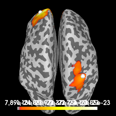
This effect can be so strong, that it completely obscures nearby coherent sources. A good tactic is to create a contrast between the signal+noise and noise-only conditions and look at the difference between the two.

one_to_all_contrast = one_to_all - one_to_all_noise

# Plot the coherence values on the cortex
brain = one_to_all_contrast.plot(
    "sample",
    subjects_dir=subjects_dir,
    hemi="both",
    figure=5,
    size=400,
    time_viewer=False,
    title="One-to-all coherence (contrast)",
)

# Indicate the true locations of the source activity on the plot (in white)
brain.add_foci(source_vert1, coords_as_verts=True, hemi="lh")
brain.add_foci(source_vert2, coords_as_verts=True, hemi="rh")

# Also indicate our chosen reference point (in red).
brain.add_foci(ref_vert, coords_as_verts=True, hemi=hemi, color=(1, 0, 0))

# Rotate the view
brain.show_view(azimuth=0, elevation=0, distance=550, focalpoint=(0, 0, 0))

fmax=0.7620232456248608
fmax=0.7620232456248608

We now see the areas that have more coherence with the reference point during the signal+noise trial than during our noise-only trial. You can see the coherence around the reference point is roughly the same during both conditions and disappears from the plot, leaving only the first simulated source.

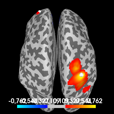
All-to-all connectivity

Finally, let’s see if we can find our two coherent sources using an all-to-all connectivity approach. We compute connectivity between all brain regions and see which regions have the most coherent activity (this should be the regions encompassing the two simulated sources).

This can be a demanding computation and to save time in this tutorial, we’re going to use a forward model that defines less source points.

# Load an oct-4 forward model that has only a few source points
fwd_lim = mne.read_forward_solution(fwd_lim_fname)

# Restrict the forward model to gradiometers only
fwd_lim = mne.pick_types_forward(fwd_lim, meg="grad", eeg=False, exclude="bads")
fwd_lim = forward_to_tangential(fwd_lim)

To reduce the number of coherence computations even further, we’re going to ignore all connections that span less than 5 centimeters.

pairs = all_to_all_connectivity_pairs(fwd_lim, min_dist=0.05)
print("There are now %d connectivity pairs" % len(pairs[0]))

There are now 96313 connectivity pairs

Compute coherence between all defined pairs using DICS. This connectivity estimate will be dominated by local field spread effects, unless we make a contrast between two conditions.

con_noise = dics_connectivity(pairs, fwd_lim, csd_noise)
con_signal = dics_connectivity(pairs, fwd_lim, csd_signal)
con_contrast = con_signal - con_noise

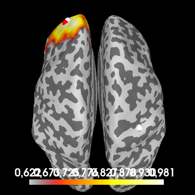
# Create a cortical map, where the "signal" at each point is the maximum
# coherence across all outgoing and incoming connections from and to that
# point.
all_to_all = con_contrast.make_stc("absmax")

brain = all_to_all.plot(
    "sample",
    subjects_dir=subjects_dir,
    hemi="both",
    figure=6,
    size=400,
    time_viewer=False,
    clim=dict(kind="value", lims=(0.5, 0.8, 1)),
    title="All-to-all coherence (contrast)",
)

# Indicate the true locations of the source activity on the plot.
brain.add_foci(source_vert1, coords_as_verts=True, hemi="lh")
brain.add_foci(source_vert2, coords_as_verts=True, hemi="rh")

# Rotate the view
brain.show_view(azimuth=0, elevation=0, distance=550, focalpoint=(0, 0, 0))

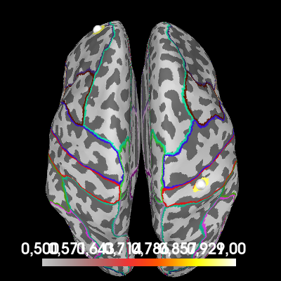
# Annotate the cortex with parcels from the "aparc" brain atlas provided by
# FreeSurfer. This is to cross reference this plot with the connectivity
# diagram we make later.
brain.add_annotation("aparc")

fmax=1.0
fmax=1.0

We see that the areas surrounding our simulated sources increase their coherence with other regions between the noise-only and noise+signal conditions. To visualize which regions are “connected” by this increased coherence, we can use a connectivity diagram.

First, we summarize our all-to-all connectivity estimate in rough parcels, provided by FreeSurfer’s “aparc” brain atlas. We plotted this atlas on the previous plot. Then, we use this is a basis for a connectivity diagram, where you can cross-reference the labels with the atlas plotted on the cortex.

# Load the parcels defined by "aparc"
labels = mne.read_labels_from_annot("sample", "aparc", subjects_dir=subjects_dir)

# Summarize the connectivity by choosing the strongest connection for each
# parcel-to-parcel combination.
p = con_contrast.parcellate(labels, "absmax", weight_by_degree=False)

# Visualize the resulting connectivity summary using a connectivity diagram.
# Show only the strongest connection.
p.plot(n_lines=1, vmin=0, vmax=1)
plt.title("Strongest parcel-to-parcel connection", color="white")

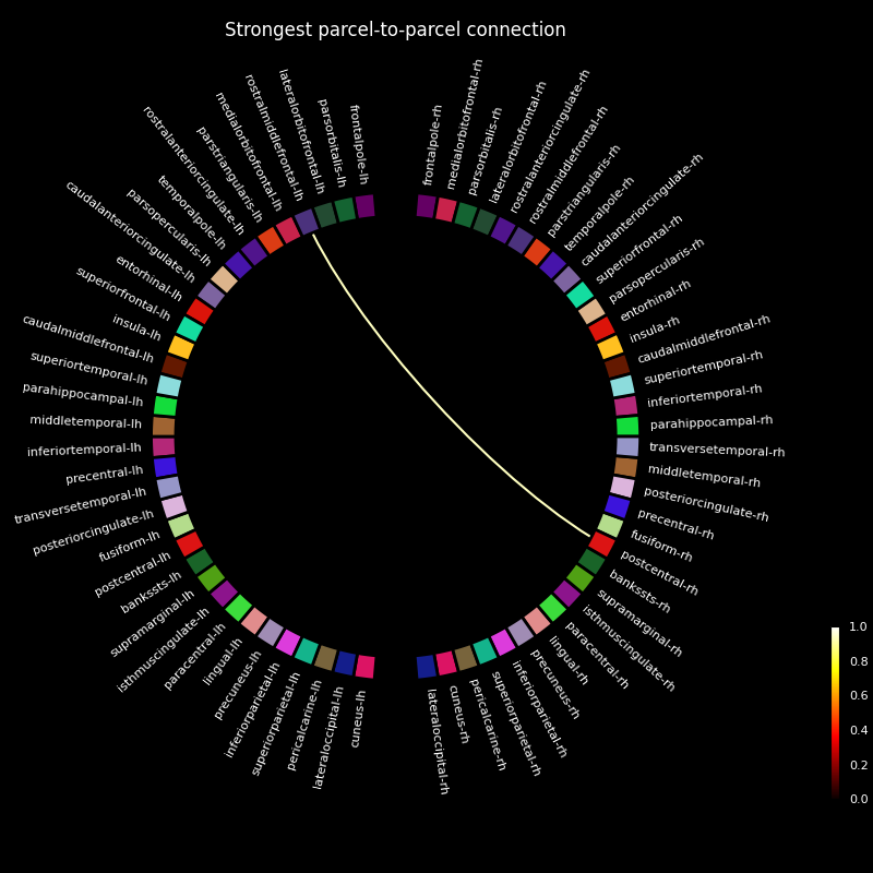
Text(0.5, 1.0, 'Strongest parcel-to-parcel connection')

While each parcel-parcel combination has a non-zero coherence with each other, we find that the strongest connection is between the parcels encompassing our simulated sources.

When analyzing real measurement data from multiple subjects, we can use statistics to define a threshold to prune the connectivity estimate [3].

References

[1]

Fries, P. (2015). Rhythms for Cognition: Communication through Coherence. Neuron, 88(1), 220–235. https://doi.org/10.1016/j.neuron.2015.09.034

[2]

Gross, J., Kujala, J., Hamalainen, M., Timmermann, L., Schnitzler, A., & Salmelin, R. (2001). Dynamic imaging of coherent sources: Studying neural interactions in the human brain. Proceedings of the National Academy of Sciences, 98(2), 694–699. https://doi.org/10.1073/pnas.98.2.694

[3] (1,2)

van Vliet, M., Liljeström, M., Aro, S., Salmelin, R. and Kujala, J. (2018). “Functional connectivity analysis using DICS: from raw MEG data to group-level statistics in Python”. bioRxiv 245530. https://doi.org/10.1101/245530