Tools
This is the documentation for the friction_tools module (download).
This module contains a set of high-level routines for constructing a
simulation.
The simulation is contained in the class friction_tools.FrictionSimulation,
and most routines are methods of this class.
The simulated structure is built as an ASE Atoms objects,
stored as the variable system, and interactions are
handled as a Pysic calculator stored as the variable calc.
It is possible to directly access these object for
complete control of the simulation.
The FrictionSimulation class
System setup
friction_tools.FrictionSimulation.create_slab()friction_tools.FrictionSimulation.create_atoms()friction_tools.FrictionSimulation.create_random_atoms()friction_tools.FrictionSimulation.duplicate_atoms()friction_tools.FrictionSimulation.remove_atoms()friction_tools.FrictionSimulation.create_interaction()friction_tools.FrictionSimulation.attach_with_springs()friction_tools.FrictionSimulation.continue_from_trajectory()friction_tools.FrictionSimulation.set_temperature()friction_tools.FrictionSimulation.set_velocities()friction_tools.FrictionSimulation.create_dynamics()friction_tools.FrictionSimulation.run_simulation()
Constraints
friction_tools.FrictionSimulation.fix_positions()friction_tools.FrictionSimulation.fix_velocities()friction_tools.FrictionSimulation.fix_positions_on_line()friction_tools.FrictionSimulation.fix_positions_on_plane()friction_tools.FrictionSimulation.add_constant_force()friction_tools.FrictionSimulation.remove_constraints()
Output
friction_tools.FrictionSimulation.list_atoms()friction_tools.FrictionSimulation.calculate_potential_energy()friction_tools.FrictionSimulation.print_stats()friction_tools.FrictionSimulation.write_positions_to_file()friction_tools.FrictionSimulation.write_average_position_to_file()friction_tools.FrictionSimulation.write_velocities_to_file()friction_tools.FrictionSimulation.write_average_velocities_to_file()friction_tools.FrictionSimulation.write_forces_to_file()friction_tools.FrictionSimulation.write_average_force_to_file()friction_tools.FrictionSimulation.write_energy_and_temperature_to_file()friction_tools.FrictionSimulation.take_snapshot()friction_tools.FrictionSimulation.write_xyzfile()
Automated output
friction_tools.FrictionSimulation.print_stats_during_simulation()friction_tools.FrictionSimulation.gather_positions_during_simulation()friction_tools.FrictionSimulation.gather_average_position_during_simulation()friction_tools.FrictionSimulation.gather_velocities_during_simulation()friction_tools.FrictionSimulation.gather_average_velocities_during_simulation()friction_tools.FrictionSimulation.gather_forces_during_simulation()friction_tools.FrictionSimulation.gather_average_force_during_simulation()friction_tools.FrictionSimulation.gather_energy_and_temperature_during_simulation()friction_tools.FrictionSimulation.gather_work_during_simulation()friction_tools.FrictionSimulation.gather_total_work_during_simulation()friction_tools.FrictionSimulation.save_trajectory_during_simulation()friction_tools.FrictionSimulation.take_snapshots_during_simulation()
Analysis
Tools functions
Array manipulation
friction_tools.add_arrays_by_component()friction_tools.add_to_array()friction_tools.calculate_column_maxima()friction_tools.calculate_column_minima()friction_tools.calculate_column_norms()friction_tools.calculate_column_sums()friction_tools.calculate_row_maxima()friction_tools.calculate_row_minima()friction_tools.calculate_row_norms()friction_tools.calculate_row_sums()friction_tools.concatenate_arrays_by_columns()friction_tools.concatenate_arrays_by_rows()friction_tools.create_array()friction_tools.crop_array()friction_tools.divide_arrays_by_component()friction_tools.multiply_array()friction_tools.multiply_arrays_by_component()friction_tools.shift_array_by_columns()friction_tools.shift_array_by_rows()friction_tools.subtract_arrays_by_component()
Output
friction_tools.write_array_to_file()friction_tools.trajectory_to_xyz()friction_tools.append_file()friction_tools.write_file()
Load data
Plot
Module API
A module containing routines for setting up simple friction simulations.
-
class
friction_tools.FixLine(indices, direction)[source]¶ A constraint class for fixing atomic positions on a line
-
class
friction_tools.FixPlane(indices, normal)[source]¶ A constraint class for fixing atomic positions in a plane
-
class
friction_tools.FixPositions(indices, fixed)[source]¶ A constraint class for fixing atomic positions
-
class
friction_tools.FixVelocities(indices, velocity, dt, fixed)[source]¶ A constraint class for fixing atomic velocities
-
class
friction_tools.FrictionSimulation[source]¶ A class defining a simulation environment.
The class contains convenient methods for setting up a simulation.
-
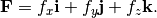
add_constant_force(indices, force)[source]¶ Adds a constant external force on atoms.
Adds an external force on the specified atoms
Parameters:
- indices: list of integers
- the indices of the atoms to be constrained - note that Python indexing starts from 0
- force: list of three floats
- the force
[fx, fy, fz]to be applied on the given atoms
-
attach_with_springs(index_list1, index_list2, strength, cutoff=5.0)[source]¶ Attaches the atoms from one list with the atoms in another list with springs.
The two lists of atoms need to have an equal number of atoms,
 , and the
method will create harmonic interactions between the listed atoms such that the
atoms are connected in order: for
, and the
method will create harmonic interactions between the listed atoms such that the
atoms are connected in order: for index_list1 = [0, 1, 2],index_list2 = [3, 4, 5]( ),
the interactions will be created for pairs 0-3, 1-4, and 2-5.
),
the interactions will be created for pairs 0-3, 1-4, and 2-5.The potential energy of the interaction is
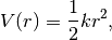
where
 is the distance between the atoms. That means the equilibrium
distance is 0. You can use the method, for instance, to create harmonic potential
wells for atoms by attaching them to constrained ghost atoms.
is the distance between the atoms. That means the equilibrium
distance is 0. You can use the method, for instance, to create harmonic potential
wells for atoms by attaching them to constrained ghost atoms.Parameters:
- index_list1: integer list
- indices of atoms to be connected
- index_list2: integer list
- indices of atoms list1 is being connected to
- strength: real number
- strength of the attachment, spring constant
- cutoff: real number
- cutoff for the interaction - if the atoms are farther away from each other than this, the potential is ignored. cutoff is restricted to cutoff < cell_width (default 10.0) because otherwise springs would be attached to periodic replicas as well.
-
continue_from_trajectory(filename='simulation.traj', frame=-1)[source]¶ Read the system geometry from a previously saved trajectory.
Parameters:
- filename: string
- name of the trajectory file to be read
- frame: integer
- the number of the configuration to be read. by default this is -1, meaning the last configuration of the trajectory is read.
-
create_atoms(element, positions)[source]¶ Creates atoms of the given element in the given positions.
The atoms are stored in
tools.FrictionSimulation.pieces. Once you’ve added all the pieces you need, finalize the system withtools.FrictionSimulation.finalize_system().Parameters:
- element: string
- the chemical symbol of the atoms, e.g., ‘C’
- positions: array of real numbers
- the xyz coordinates of the atoms, in an array, e.g.,
[[0, 0, 0], [1, 1, 1]]
-
create_dynamics(dt=2.0, temperature=None, coupled_indices=None, strength=0.01)[source]¶ Defines the type of molecular dynamics to be run.
By default, energy conserving dynamics are run, i.e, the microcanonical ensemble is used. That is, the normal Velocity Verlet algorithm is applied.
NVT dynamics are run if the argument
temperatureis given. (NVT: number of particles, volume, and temperature are kept constant - temperature only approximately.) This is done using Langevin dynamics.This Langevin thermostat adds a fictious friction force and a random noise force on all atoms. This may lead to computational artifacts if there is collective motion. It’s especially important not to apply the thermostat on atoms which are being dragged or move at a fixed velocity, as the thermostat will add artificial friction on them. In order to select the atoms which are being affected by the thermostat, you can specify their indices as a list with the
coupled_indicesargument.- Note The atomic structure cannot be altered after this method is called (if temperature is set). Create all the atoms before calling this.
Parameters:
- dt: real number
- timestep
 used in integrating the equations of motion, in fs - 2 fs by default.
 - temperature: real number
- temperature in K, if you wish to apply a thermostat
- coupled_indices: integer list
- indices of the atoms the thermostat affects
- strength: real number
- strength of the thermostat, larger number meaning a stronger deviation from Newtonian mechanics - 0.01 by default
-
create_graphite()[source]¶ Creates a graphite structure.
The slab is 2D infinite in xy-plane, its surfaces exposed in the z-direction. The structure is FCC, see e.g. http://en.wikipedia.org/wiki/Face_Centered_Cubic
Parameters:
- element: string
- the chemical symbol for the atoms of the slab, e.g., ‘Au’
- bottom_z: real number
- the z-coordinate of the lower surface of the slab
- top_z: real number
- the z-coordinate of the top surface of the slab
- xy_cells: integer
- the number of lattice cells to be created in x and y directions - as the
width of the simulation box is determined by the
FrictionSimulation(‘cell_width’), this will determine the lattice constant - z_cells: integer
- the number of lattice cells to be created in z direction
-
create_graphite2()[source]¶ Creates a graphite structure.
The slab is 2D infinite in xy-plane, its surfaces exposed in the z-direction. The structure is FCC, see e.g. http://en.wikipedia.org/wiki/Face_Centered_Cubic
Parameters:
- element: string
- the chemical symbol for the atoms of the slab, e.g., ‘Au’
- bottom_z: real number
- the z-coordinate of the lower surface of the slab
- top_z: real number
- the z-coordinate of the top surface of the slab
- xy_cells: integer
- the number of lattice cells to be created in x and y directions - as the
width of the simulation box is determined by the
FrictionSimulation(‘cell_width’), this will determine the lattice constant - z_cells: integer
- the number of lattice cells to be created in z direction
-
create_interaction(element_pair, strength, equilibrium_distance, type='LJ')[source]¶ Creates an interaction between the two given types of atoms.
The interactions are described by the simple Lennard-Jones potential (http://en.wikipedia.org/wiki/Lennard-Jones_potential)
![V(r) = \varepsilon \left[ \left( \frac{\sigma}{r} \right)^12 - \left( \frac{\sigma}{r} \right)^6 \right]](_images/math/6b93d3f1555e9b0f539a2cdca66da48267df8ec0.png)
This is not a realistic interaction except for some very special cases such as noble gases. However, it is simple and will work fine as a placeholder.
The method creates an interaction between two types of atoms as defined by
element_pair. The types may be the same, so for instance if you have'Au'atoms in your system, you can make them interact withcreate_interaction( ['Au', 'Au'], ...)Parameters:
- element_pair: string list
- the types that will interact, e.g,
['Au', 'Au']or['B', 'C'] - strength: real number
- the depth of the potential energy minimum (
 ) for the pair interaction, in eV
 - equilibrium_distance: real number
- the atomic distance, , at which
 has its minimum
-
create_random_atoms(number, element, bottom_z, top_z, minimum_distance=2.0)[source]¶ Adds the given number of atoms randomly in a given volume.
The atoms are added randomly and for each added atom it is checked that it is not too close to previously added atoms. If you try to insert too many atoms, there will not be enough room and the algorithm stops after failing for long enough.
Parameters:
- number: integer
- the number of atoms to add
- element: string
- the chemical symbol of the atoms, e.g., ‘C’
- bottom_z: real number
- the minimum z coordinate the atoms may get
- top_z: real number
- the maximum z coordinate the atoms may get
- minimum_distance: real number
- the minimum allowed separation between the added atoms
-
create_slab(element, bottom_z=0.0, top_z=None, z_cells=3, xy_cells=4)[source]¶ Creates a slab of atoms in the FCC (face-centered cubic) lattice structure.
The slab is 2D infinite in xy-plane, its surfaces exposed in the z-direction. The structure is FCC, see e.g. http://en.wikipedia.org/wiki/Face_Centered_Cubic
Parameters:
- element: string
- the chemical symbol for the atoms of the slab, e.g., ‘Au’
- bottom_z: real number
- the z-coordinate of the lower surface of the slab
- top_z: real number
- the z-coordinate of the top surface of the slab
- xy_cells: integer
- the number of lattice cells to be created in x and y directions - as the
width of the simulation box is determined by the
FrictionSimulation(‘cell_width’), this will determine the lattice constant - z_cells: integer
- the number of lattice cells to be created in z direction
-
duplicate_atoms(element, indices)[source]¶ Creates a set of atoms with the same positions as the atoms with the given indices.
The new atoms will be of the given element. This function can be used to create ghost atoms to be used with
attach_with_springs()or duplicate parts of the system to be moved in the correct place withmove_atoms()Parameters:
- element: string
- the chemical symbol of the atoms, e.g., ‘C’
- indices: integer list
- indices of the atoms to be copied
-
fix_positions(indices, xyz=[True, True, True])[source]¶ Constrains the positions of particles.
- Note call this method before running the simulation with
tools.FrictionSimulation.run_simulation()
This method freezes coordinates of the atoms whose indices are given. By default, the atoms are not allowed to move at all, but the optional argument
xyzallows one to freeze only some coordinates. For example:>>> from friction_tools import * >>> s = FrictionSimulation() >>> # define the system... >>> s.fix_positions(indices=[...], xyz=[True,True,False])
freezes the x and y coordinates of the specified atoms (
xyz = [True,True,False]).Parameters:
- indices: list of integers
- the indices of the atoms to be constrained - note that Python indexing starts from 0
- xyz: list of three booleans
- logical tags specifying if the xyz coordinates are fixed (
Truemeans the coordinate is fixed)
- Note call this method before running the simulation with
-
fix_positions_on_line(indices, direction)[source]¶ Constrains the positions of particles on a line.
- Note call this method before running the simulation with
tools.FrictionSimulation.run_simulation()
This method constrains coordinates of the atoms whose indices are given on a line. The line is defined by the given direction
 and the initial position
of the particle
and the initial position
of the particle  .
.
Parameters:
- indices: list of integers
- the indices of the atoms to be constrained - note that Python indexing starts from 0
- direction: list of three floats
- the direction
[ux, uy, uz]in which the particles are allowed to move
- Note call this method before running the simulation with
-
fix_positions_on_plane(indices, normal)[source]¶ Constrains the positions of particles on a plane.
- Note call this method before running the simulation with
tools.FrictionSimulation.run_simulation()
This method constrains coordinates of the atoms whose indices are given on a plane. The plane is defined by the given normal
 and the initial position
of the particle .
and the initial position
of the particle .
Parameters:
- indices: list of integers
- the indices of the atoms to be constrained - note that Python indexing starts from 0
- normal: list of three floats
- the normal vector
[nx, ny, nz]to the plane in which the particles are allowed to move
- Note call this method before running the simulation with
-
fix_velocities(indices, velocity, xyz=[True, True, True])[source]¶ Constrains the velocities of particles.
- Note call this method before running the simulation with
tools.FrictionSimulation.run_simulation()
This method freezes velocities of the atoms whose indices are given. By default, the atoms move with constant velocity, but the optional argument
xyzallows one to fix only a given component of force. For example:>>> from tools import * >>> s = FrictionSimulation() >>> # define the system... >>> s.fix_velocities(indices=[...], velocity=[0.01,0.0,0.0], xyz=[True,False,True])
fixes the velocities in x and z directions to
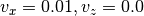 Å/fs
(
Å/fs
(xyz = [True,False,True]) but allows the velocity to change freely in the y direction.Parameters:
- indices: list of integers
- the indices of the atoms to be constrained - note that Python indexing starts from 0
- velocity: list of three floats
- the velocity given to the particles
- xyz: list of three booleans
- logical tags specifying if the xyz coordinates are fixed (
Truemeans the coordinate is fixed)
- Note call this method before running the simulation with
-
gather_average_force_during_simulation(interval=100, filename='avr_force.txt', indices=None)[source]¶ Makes the simulator write averages of instantaneous forces of atoms during simulation.
- Note call this method before running the simulation with
tools.FrictionSimulation.run_simulation()
The format is:
(f_x) (f_y) (f_z)
This method instructs the simulator to call
tools.FrictionSimulation.write_average_force_to_file()periodically during the molecular dynamics run, everyintervalsteps.The data is written in a single file where each line represents a point in the time series.
Parameters:
- interval: integer
- the number of MD steps between consecutive information writing
- filename: string
- name of the file where the data is written
- indices: list of integers
- the indices of the atoms to be constrained - note that Python indexing starts from 0. By default, all atoms are included.
- Note call this method before running the simulation with
-
gather_average_position_during_simulation(interval=100, filename='avr_position.txt', indices=None)[source]¶ Makes the simulator write averages of positions of atoms during simulation.
- Note call this method before running the simulation with
tools.FrictionSimulation.run_simulation()
The format is:
(x) (y) (z)
This method instructs the simulator to call
tools.FrictionSimulation.write_average_position_to_file()periodically during the molecular dynamics run, everyintervalsteps.The data is written in a single file where each line represents a point in the time series.
Parameters:
- interval: integer
- the number of MD steps between consecutive information writing
- filename: string
- name of the file where the data is written
- indices: list of integers
- the indices of the atoms to be constrained - note that Python indexing starts from 0. By default, all atoms are included.
- Note call this method before running the simulation with
-
gather_average_velocities_during_simulation(interval=10, filename='avr_velocities.txt', indices=None)[source]¶ Makes the simulator write average velocities of atoms during simulation.
- Note call this method before running the simulation with
tools.FrictionSimulation.run_simulation()
The format is:
(atom 0 v_x) (atom 0 v_y) (atom 0 v_z)
(atom 1 v_x) (atom 1 v_y) (atom 1 v_z)
(atom 2 v_x) (atom 2 v_y) (atom 2 v_z)
...
This method instructs the simulator to call
tools.FrictionSimulation.write_average_velocities_to_file()periodically during the molecular dynamics run, everyintervalsteps.The average velocities recorded are the averages since the previous recording. So, when writing at intervals of
 ,
the average velocity of atom
,
the average velocity of atom  at time
  will be the atomic displacement
 divided by the elapsed time
 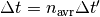 , with
  being
the MD timestep:
being
the MD timestep: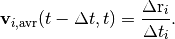
The given filename is automatically modified to include the current MD step number. For instance, if the filename is given as
data.txt, the data from, say, step 20 will be written to filedata00020.txt.Parameters:
- interval: integer
- the number of MD steps between consecutive information writing
- filename: string
- name of the file where the data is written
- indices: list of integers
- the indices of the atoms to be constrained - note that Python indexing starts from 0. By default, all atoms are included.
- Note call this method before running the simulation with
-
gather_energy_and_temperature_during_simulation(interval=100, filename='energy.txt')[source]¶ Makes the simulator write energy and temperature during simulation.
- Note call this method before running the simulation with
tools.FrictionSimulation.run_simulation()
The format is:
(potential energy) (kinetic energy) (total energy) (temperature)
This method instructs the simulator to call
tools.FrictionSimulation.write_energy_and_temperature_to_file()periodically during the molecular dynamics run, everyintervalsteps.The data is written in a single file where each line represents a point in the time series.
Parameters:
- interval: integer
- the number of MD steps between consecutive information writing
- filename: string
- name of the file where the data is written
- Note call this method before running the simulation with
-
gather_forces_during_simulation(interval=100, filename='forces.txt', indices=None)[source]¶ Makes the simulator write instantaneous forces of atoms during simulation.
- Note call this method before running the simulation with
tools.FrictionSimulation.run_simulation()
The format is:
(atom 0 f_x) (atom 0 f_y) (atom 0 f_z)
(atom 1 f_x) (atom 1 f_y) (atom 1 f_z)
(atom 2 f_x) (atom 2 f_y) (atom 2 f_z)
...
This method instructs the simulator to call
tools.FrictionSimulation.write_forces_to_file()periodically during the molecular dynamics run, everyintervalsteps.The given filename is automatically modified to include the current MD step number. For instance, if the filename is given as
data.txt, the data from, say, step 20 will be written to filedata00020.txt.Parameters:
- interval: integer
- the number of MD steps between consecutive information writing
- filename: string
- name of the file where the data is written
- indices: list of integers
- the indices of the atoms to be constrained - note that Python indexing starts from 0. By default, all atoms are included.
- Note call this method before running the simulation with
-
gather_positions_during_simulation(interval=10, filename='positions.txt', indices=None)[source]¶ Makes the simulator write coordinates of atoms during simulation.
The format is:
(atom 0 x) (atom 0 y) (atom 0 z)
(atom 1 x) (atom 1 y) (atom 1 z)
(atom 2 x) (atom 2 y) (atom 2 z)
...
- Note call this method before running the simulation with
tools.FrictionSimulation.run_simulation()
This method instructs the simulator to call
tools.FrictionSimulation.write_positions_to_file()periodically during the molecular dynamics run, everyintervalsteps.The given filename is automatically modified to include the current MD step number. For instance, if the filename is given as
data.txt, the data from, say, step 20 will be written to filedata00020.txt.Parameters:
- interval: integer
- the number of MD steps between consecutive information writing
- filename: string
- name of the file where the data is written
- indices: list of integers
- the indices of the atoms to be constrained - note that Python indexing starts from 0. By default, all atoms are included.
- Note call this method before running the simulation with
-
gather_total_work_during_simulation(interval=100, filename='total_work.txt', indices=None)[source]¶ Makes the simulator write the total work done on atoms during simulation.
- Note call this method before running the simulation with
tools.FrictionSimulation.run_simulation()
This method instructs the simulator to call
tools.FrictionSimulation.write_total_work_to_file()periodically during the molecular dynamics run, everyintervalsteps.The data is written in a single file where each line represents a point in the time series.
Parameters:
- interval: integer
- the number of MD steps between consecutive information writing
- filename: string
- name of the file where the data is written
- indices: list of integers
- the indices of the atoms to be constrained - note that Python indexing starts from 0. By default, all atoms are included.
- Note call this method before running the simulation with
-
gather_velocities_during_simulation(interval=10, filename='velocities.txt', indices=None)[source]¶ Makes the simulator write instantaneous velocities of atoms during simulation.
- Note call this method before running the simulation with
tools.FrictionSimulation.run_simulation() - Note Due to a bug/feature in ASE, if you fix the velocities of atoms with
tools.FrictionSimulation.fix_velocities(), the velocities for these atoms are reported to be 0.0. The methodtools.FrictionSimulation.gather_average_velocities_during_simulation()does report the correct average velocities for all atoms though.
The format is:
(atom 0 v_x) (atom 0 v_y) (atom 0 v_z)
(atom 1 v_x) (atom 1 v_y) (atom 1 v_z)
(atom 2 v_x) (atom 2 v_y) (atom 2 v_z)
...
This method instructs the simulator to call
tools.FrictionSimulation.write_velocities_to_file()periodically during the molecular dynamics run, everyintervalsteps.The given filename is automatically modified to include the current MD step number. For instance, if the filename is given as
data.txt, the data from, say, step 20 will be written to filedata00020.txt.Parameters:
- interval: integer
- the number of MD steps between consecutive information writing
- filename: string
- name of the file where the data is written
- indices: list of integers
- the indices of the atoms to be constrained - note that Python indexing starts from 0. By default, all atoms are included.
- Note call this method before running the simulation with
-
gather_work_during_simulation(interval=100, filename='work.txt', indices=None)[source]¶ Makes the simulator write work done on atoms during simulation.
- Note call this method before running the simulation with
tools.FrictionSimulation.run_simulation()
The format is:
(atom 0 work)
(atom 1 work)
(atom 2 work)
...
This method instructs the simulator to call
tools.FrictionSimulation.write_work_to_file()periodically during the molecular dynamics run, everyintervalsteps.Work is defined as the line integral of the force. The recorded values are the work done on each individual atom since the previous recording.
So, when writing at intervals of
, the work on atom
at time is
with
, being
the MD timestep.The given filename is automatically modified to include the current MD step number. For instance, if the filename is given as
data.txt, the data from, say, step 20 will be written to filedata00020.txt.Parameters:
- interval: integer
- the number of MD steps between consecutive information writing
- filename: string
- name of the file where the data is written
- indices: list of integers
- the indices of the atoms to be constrained - note that Python indexing starts from 0. By default, all atoms are included.
- Note call this method before running the simulation with
-
get_indices_by_element(element)[source]¶ Returns the indices of atoms of given element.
Parameters:
- element: string
- the chemical symbol of the atoms, e.g., ‘C’
-
get_indices_z_less_than(z_limit)[source]¶ Returns the indices of the atoms whose z-coordinate is less than the given value, as a list.
This can be used for easily finding, e.g., the bottom of a slab.
Parameters:
- z_limit: float
- the limiting z value
-
get_indices_z_more_than(z_limit)[source]¶ Returns the indices of the atoms whose z-coordinate is more than the given value, as a list.
This can be used for easily finding, e.g., the top of a slab.
Parameters:
- z_limit: float
- the limiting z value
-
load_state_from_trajectory(step=-1, filename='simulation.traj')[source]¶ Loads the geometry from a saved trajectory.
If you have a saved trajectory from
tools.FrictionSimulation.save_trajectory_during_simulation(), this method can be used for reading in a state from the trajectory.Parameters:
- step: integer
- the timestep which is restored - by default the last recorded state is chosen
- filename: string
- name of the trajectory file
-
print_stats(time_it=False)[source]¶ Prints the energy and temperature information in human readable format.
Parameters:
- time_it: boolean
- if
True, the calculation is timed and the execution time is printed
-
print_stats_during_simulation(interval=10)[source]¶ Makes the simulator print energies and temperature during simulation.
- Note call this method before running the simulation with
tools.FrictionSimulation.run_simulation()
This method instructs the simulator to call
tools.FrictionSimulation.print_stats()periodically during the molecular dynamics run, everyintervalsteps. This is a convenient way to monitor the progress of your simulation.Parameters:
- interval: integer
- the number of MD steps between consecutive information writing
- Note call this method before running the simulation with
-
remove_atoms(indices)[source]¶ Removes atoms with the given indices.
Parameters:
- indices: integer list
- indices of the atoms to be removed
-
run_simulation(time=10, steps=None)[source]¶ Runs molecular dynamics (MD).
This method executes the actual simulation according to the parameters defined earlier by other methods.
The simulation may take a long time to run, so it is a very good idea to first run a short test run to get an idea on the execution time. You can time the simulation with:
>>> from tools import *
>>> s = FrictionSimulation()
>>> # define the system...
>>> import time
>>> t0 = time.time()
>>> s.run_simulation(steps=5)
>>> t1 = time.time()
>>> print "The simulation took "+str(t1-t0)+" s."
The simulation runs for a given length of time, which can be defined as either simulated time or number of molecular dynamics steps. If the argument
stepsis given, the simulation runs for this many steps. Iftimeis given, the simulation is run for this long (in fs). Even if time is
specified, the simulation length is still determined in steps  ,
where is the timestep.
,
where is the timestep.Parameters:
- time: float
- simulation time in fs, 10 fs by default
- steps: integer
- simulation time in MD steps
-
save_trajectory_during_simulation(interval=100, filename='simulation.traj')[source]¶ Saves the simulation trajectory in binary format.
- Note call this method before running the simulation with
tools.FrictionSimulation.run_simulation()
This method saves the simulation as a trajectory file, from which the positions of particles can be extracted at the different points of time of the simulation.
Parameters:
- interval: integer
- the number of MD steps between consecutive information writing
- filename: string
- name of the file where the data is written
- Note call this method before running the simulation with
-
set_temperature(temperature=50)[source]¶ Gives the atoms initial velocities according to the Maxwell-Boltzmann distribution.
The default temperature is 50 K. (Room temperature is about 300 K.)
Parameters:
- temperature: float
- the initial temperature in K - 50 K by default
-
set_velocities(velocity, indices)[source]¶ Gives the atoms initial velocities.
You must give the indices of the atoms whose velocities you are defining as a list. If all the atoms should receive the same velocity,
velocitycan be a single vector. You can also, instead, give a list of velocities to define the velocities one by one. In that case, the length of the velocity and index lists must match.Parameters:
- velocity: real vector or a list of vectors
- the velocity or velocities of th atoms
- indices: integer list
- the indices of the atoms affected
-
take_snapshot(filename='snapshot.png', addStepNumber=False)[source]¶ Makes a png format snapshot of the system.
Parameters:
- filename: string
- name of the trajectory file
- addStepNumber: boolean
- meant for internal use - if
True, adds the MD step number in the filename to prevent overwriting
-
take_snapshots_during_simulation(interval=100, filename='snapshot.png')[source]¶ Takes png-format snapshots of the system during the simulation.
- Note call this method before running the simulation with
tools.FrictionSimulation.run_simulation()
This method generates images of the system in png format.
Parameters:
- interval: integer
- the number of MD steps between consecutive information writing
- filename: string
- name of the file where the data is written
- Note call this method before running the simulation with
-
write_average_force_to_file(filename='force_sum.txt', indices=None)[source]¶ Writes the average of instantaneous forces of the atoms in a file.
The format is:
(f_x) (f_y) (f_z)
...
Parameters:
- filename: string
- name of the file where the information is written
- indices: list of integers
- the indices of the atoms whose info is to be written - note that Python indexing starts from 0. By default all atoms are included
-
write_average_position_to_file(filename='avr_position.txt', indices=None)[source]¶ Writes the mean of the coordinates of the atoms in a file.
The format is:
(x) (y) (z)
Parameters:
- filename: string
- name of the file where the information is written
- indices: list of integers
- the indices of the atoms whose info is to be written - note that Python indexing starts from 0. By default all atoms are included
-
write_average_velocities_to_file(dt, filename='avr_velocities.txt', indices=None, addStepNumber=False)[source]¶ For internal use. Writes the average velocities of the atoms in a file.
The format is:
(atom 0 v_x) (atom 0 v_y) (atom 0 v_z)
(atom 1 v_x) (atom 1 v_y) (atom 1 v_z)
(atom 2 v_x) (atom 2 v_y) (atom 2 v_z)
...
Parameters:
- filename: string
- name of the file where the information is written
- indices: list of integers
- the indices of the atoms whose info is to be written - note that Python indexing starts from 0. By default all atoms are included
- addStepNumber: boolean
- meant for internal use - if
True, adds the MD step number in the filename to prevent overwriting
-
write_energy_and_temperature_to_file(filename='energies.txt')[source]¶ Appends the instantaneous energy and temperature information in a file.
The format is:
(potential energy) (kinetic energy) (total energy) (temperature)
Since this method does not write atom-by-atom information, it does not create a new file but appends its output at the end of the specified file.
Parameters:
- filename: string
- name of the file where the information is written
-
write_forces_to_file(filename='forces.txt', indices=None, addStepNumber=False)[source]¶ Writes the instantaneous forces of the atoms in a file.
The format is:
(atom 0 f_x) (atom 0 f_y) (atom 0 f_z)
(atom 1 f_x) (atom 1 f_y) (atom 1 f_z)
(atom 2 f_x) (atom 2 f_y) (atom 2 f_z)
...
Parameters:
- filename: string
- name of the file where the information is written
- indices: list of integers
- the indices of the atoms whose info is to be written - note that Python indexing starts from 0. By default all atoms are included
- addStepNumber: boolean
- meant for internal use - if
True, adds the MD step number in the filename to prevent overwriting
-
write_positions_to_file(filename='positions.txt', indices=None, addStepNumber=False)[source]¶ Writes the coordinates of the atoms in a file.
The format is:
(atom 0 x) (atom 0 y) (atom 0 z)
(atom 1 x) (atom 1 y) (atom 1 z)
(atom 2 x) (atom 2 y) (atom 2 z)
...
Parameters:
- filename: string
- name of the file where the information is written
- indices: list of integers
- the indices of the atoms whose info is to be written - note that Python indexing starts from 0. By default all atoms are included
- addStepNumber: boolean
- meant for internal use - if
True, adds the MD step number in the filename to prevent overwriting
-
write_total_work_to_file(filename='total_work.txt', indices=None)[source]¶ For internal use. Writes the work done on the atoms in a file.
Parameters:
- filename: string
- name of the file where the information is written
- indices: list of integers
- the indices of the atoms whose info is to be written - note that Python indexing starts from 0. By default all atoms are included
-
write_velocities_to_file(filename='velocities.txt', indices=None, addStepNumber=False)[source]¶ Writes the instantaneous velocities of the atoms in a file.
- Note Due to a bug/feature in ASE, if you fix the velocities of atoms with
tools.FrictionSimulation.fix_velocities(), the velocities for these atoms are reported to be 0.0. The methodtools.FrictionSimulation.gather_average_velocities_during_simulation()does report the correct average velocities for all atoms though.
The format is:
(atom 0 v_x) (atom 0 v_y) (atom 0 v_z)
(atom 1 v_x) (atom 1 v_y) (atom 1 v_z)
(atom 2 v_x) (atom 2 v_y) (atom 2 v_z)
...
Parameters:
- filename: string
- name of the file where the information is written
- indices: list of integers
- the indices of the atoms whose info is to be written - note that Python indexing starts from 0. By default all atoms are included
- addStepNumber: boolean
- meant for internal use - if
True, adds the MD step number in the filename to prevent overwriting
- Note Due to a bug/feature in ASE, if you fix the velocities of atoms with
-
write_work_to_file(filename='work.txt', indices=None, addStepNumber=False)[source]¶ For internal use. Writes the work done on the atoms in a file.
The format is:
(atom 0 work)
(atom 1 work)
(atom 2 work)
...
Parameters:
- filename: string
- name of the file where the information is written
- indices: list of integers
- the indices of the atoms whose info is to be written - note that Python indexing starts from 0. By default all atoms are included
- addStepNumber: boolean
- meant for internal use - if
True, adds the MD step number in the filename to prevent overwriting
-
write_xyzfile(filename='system.xyz')[source]¶ Makes an xyz format geometry file of the system.
XYZ is a commonly used, very simple geometry file format which includes information on the types of atoms and their coordinates. This method writes such a file based on the current simulation geometry.
XYZ files can be read with almost any atomic visualization tool.
Parameters:
- filename: string
- name of the trajectory file
-
-
friction_tools.add_arrays_by_component(array1, array2)[source]¶ Adds two arrays component by component.
Equal to
np.array(array1) + np.array(array2)Parameters:
- array1: numeric array of floats
- an array
- array2: numeric array of floats
- an array
-
friction_tools.add_to_array(array, real)[source]¶ Adds a real number to an array component by component.
Equal to
np.array(array) + realParameters:
- array: numeric array of floats
- an array
- real: float
- a number
-
friction_tools.append_file(filename, output_lines)[source]¶ Writes the given string in a file.
Note that you should provide only a single string. If you want to split the output to several lines, use the newline character ‘n’.
This function does not overwrite a file, but appends the output at the end.
Parameters:
- filename: string
- name of the file to be written
- output_lines: string
- the string to be written
-
friction_tools.calculate_column_maxima(array)[source]¶ Finds the maxima for all the columns of a 2D array and returns a row 1D array containing the results.
Parameters:
- array: numeric array
- the array to be manipulated
-
friction_tools.calculate_column_minima(array)[source]¶ Finds the minima for all the columns of a 2D array and returns a row 1D array containing the results.
Parameters:
- array: numeric array
- the array to be manipulated
-
friction_tools.calculate_column_norms(array)[source]¶ Calculates euclidian norms for all the columns of a 2D array and returns a row 1D array containing the results.
Parameters:
- array: numeric array
- the array to be manipulated
-
friction_tools.calculate_column_sums(array)[source]¶ Sums all the columns of a 2D array and returns a row 1D array containing the results.
Parameters:
- array: numeric array
- the array to be manipulated
-
friction_tools.calculate_row_maxima(array)[source]¶ Finds the maxima for all the rows of a 2D array and returns a row 1D array containing the results.
Parameters:
- array: numeric array
- the array to be manipulated
-
friction_tools.calculate_row_minima(array)[source]¶ Finds the minima for all the rows of a 2D array and returns a row 1D array containing the results.
Parameters:
- array: numeric array
- the array to be manipulated
-
friction_tools.calculate_row_norms(array)[source]¶ Calculates euclidian norms for all the rows of a 2D array and returns a row 1D array containing the results.
Parameters:
- array: numeric array
- the array to be manipulated
-
friction_tools.calculate_row_sums(array)[source]¶ Sums all the rows of a 2D array and returns a row 1D array containing the results.
Parameters:
- array: numeric array
- the array to be manipulated
-
friction_tools.concatenate_arrays_by_columns(array1, array2)[source]¶ Joins two arrays together by appending column by column.
Parameters:
- array1: numeric array of floats
- an array
- array2: numeric array of floats
- an array
-
friction_tools.concatenate_arrays_by_rows(array1, array2)[source]¶ Joins two arrays together by appending row by row.
Parameters:
- array1: numeric array of floats
- an array
- array2: numeric array of floats
- an array
-
friction_tools.create_array(dimensions, value=0)[source]¶ Creates an array of the given size.
Parameters:
- dimensions: list of integers
- dimensions of the array
- value: float
- the initial value for the elements of the array
-
friction_tools.crop_array(top, left, bottom, right, array)[source]¶ Crops an array (i.e., returns a subarray).
The indices for cropping should be given as arguments. The order is
top, left, bottom, right. Fortopandleft, they are the first indices to be included, whilebottomandrightare the first indices to be dropped.For instance, if you have the array:
arry = [[1, 2, 3],
        [4, 5, 6],
        [7, 8, 9]]
The top left
 array is obtained with:
>>> crop_array(0, 0, 2, 2, arry)
[[1, 2],
 [4, 5]]
The command is equivalent to:
>>> array.copy()[top:bottom,left:right]
Parameters:
- top: integer
- first index from the top to be included
- left: integer
- first integer from the left to be included
- bottom: integer
- first index from the top to be left out
- rigth: integer
- first index from the left to be left out
-
friction_tools.divide_arrays_by_component(array1, array2)[source]¶ Divides two arrays component by component.
Equal to
np.array(array1) / np.array(array2)Parameters:
- array1: numeric array of floats
- an array
- array2: numeric array of floats
- an array
-
friction_tools.hold_plots()[source]¶ Hold the plot visible.
By default, your plots will vanish from the screen after plotting. This function prevents it. The point is, you can call
tools.plot_array()several times and the generated plots will be added together and shown when you call this function.
-
friction_tools.multiply_array(array, real)[source]¶ Multiplies an array with a real number component by component.
Equal to
np.array(array) * realParameters:
- array: numeric array of floats
- an array
- real: float
- a number
-
friction_tools.multiply_arrays_by_component(array1, array2)[source]¶ Multiplies two arrays component by component.
Equal to
np.array(array1) * np.array(array2)Parameters:
- array1: numeric array of floats
- an array
- array2: numeric array of floats
- an array
-
friction_tools.plot_array(x_values, y_values=None, y_error=None, x_range=None, y_range=None)[source]¶ Plots data.
If only one column of data is given, it is plotted against a running index.
If two columns of data are given, the first is treated as x and the second as y.
Note You should also use
tools.hold_plots().Parameters:
- x_values: list of floats
- If it’s the only input given, it is treated as the y-variable. If
y_valuesis given, this is the x-variable. - y_values: list of floats
- Values of the y-variable.
- y_error: list of floats
- Values for errorbars of y.
- x_range: list of two floats
- Plotting range for x
- y_range: list of two floats
- Plotting range for y
-
friction_tools.read_array_from_file(filename)[source]¶ Parses a file and returns a numeric array of the data found.
Parameters:
- filename: string
- name of the file to be read
-
friction_tools.read_arrays_from_files(filename, starting_index, ending_index, index_step)[source]¶ Reads numeric arrays from files.
If you have run a simulation and produced files containing numeric data through the methods
gather_xxx_during_simulation, this function can be used for reading the data in Python.You should have files with names such as
positions00100.txtetc. To read them in, give the base namepositions.txtas thefilename, and the range of integers through the other arguments:starting_indexandending_indexare the first and last index to be read, respectively, whileindex_stepis the increment.Example:
>>> read_arrays_from_files('data.txt',10,100,10)
will read the files:
data00010.txt
data00020.txt
...
data00100.txt
The function returns a list containing all the arrays extracted from the files.
Parameters:
- filename: string
- the base filename to be read
- starting_index: integer
- the first index to be read
- ending_index: integer
- the last index to be read
- index_step: integer
- the increment in indices
-
friction_tools.set_random_number_seed(seed=5801)[source]¶ Initialize random number generator (RNG).
By default, the RNG is always given the same seed so that simulations are reproducible. However, if you would like to rerun simulations with different random sequences, give a new random seed here.
This affects
set_initial_temperature()andcreate_dynamics()/ if Langevin dynamics are chosen.
Parameters:
- seed: integer
- a new RNG seed
-
friction_tools.shift_array_by_columns(array, steps=1, wrap=False)[source]¶ Moves the elements in an array in by columns.
Parameters:
- array: numeric array of floats
- an array
- steps: integer
- number of rows the elements are moved
- wrap: boolean
- if
True, elements that go over the bounds of the array appear on the other side
-
friction_tools.shift_array_by_rows(array, steps=1, wrap=False)[source]¶ Moves the elements in an array by rows.
Parameters:
- array: numeric array of floats
- an array
- steps: integer
- number of rows the elements are moved
- wrap: boolean
- if
True, elements that go over the bounds of the array appear on the other side
-
friction_tools.subtract_arrays_by_component(array1, array2)[source]¶ Subtracts two arrays component by component.
Equal to
np.array(array1) - np.array(array2)Parameters:
- array1: numeric array of floats
- an array
- array2: numeric array of floats
- an array
-
friction_tools.trajectory_to_xyz(filename_in='simulation.traj', filename_out='simulation.xyz')[source]¶ Converts a trajectory file to an XYZ file.
Parameters:
- filaname_in: string
- name of the trajectory file
- filaname_out: string
- name of the XYZ file
-
friction_tools.write_array_to_file(filename, array)[source]¶ Writes an array to a file.
Note The method calls the Numpy routine:
array.tofile(filename, sep=" ", format="%20.5f")
which results in all the values stored in the array being written in one line. If you read it back in with
tools.read_array_from_file(), you get a 1D array containing the values. To fix the shape, specify it explicitly:>>> arry = [[1, 2], [3, 4]] array([[1, 2], [3, 4]]) >>> write_array_to_file(filename='array.txt', arry) >>> new_arry = read_array_from_file('array.txt') >>> new_arry array([[1, 2, 3, 4]]) >>> new_arry.shape = (2,2) >>> new_arry array([[1, 2], [3, 4]])
Parameters:
- filename: string
- name of the file to be written
- array: numeric array
- the array to be written
-
friction_tools.write_file(filename, output_lines)[source]¶ Writes the given string in a file.
Note that you should provide only a single string. If you want to split the output to several lines, use the newline character
\n.If the file exists, it is overwritten.
Parameters:
- filename: string
- name of the file to be written
- output_lines: string
- the string to be written